Zumo Segway’s Documentation¶

Introduction¶

This documentation features the implementation of the Segway behavior in a Zumo32u4 board. The process started with the modeling of the system according to the capabilities of the Zumo32u4. Therefore, a Zumo32u4 chapter was written with the relevant about the Zumo’s IMU, Zumo’s encoders and Zumo’s motos.

Secondly a model from the literature was selected. The model in [3] was firstly analyzed. The developed model in [3] was develop upon simplifying and considering it as a cart with an inverted pendulum installed on top. It defined the input as the force applied to the cart. To use this model the force had to be written in terms of the torque applied to the pendulum.

The model in [15] proved to be better applicable for implementation on a Zumo32u4 since it was in already in terms of torque applied to the pendulum system and the physical model upon the state variable model was based could be easily mapped to the Zumo by simplifying it.

None of the model in [3] and [15] considered a caterpillar driven system. Nevertheless, [15] considers explicitly the inertia moment of the wheels which can be replaced by the inertia moment of the caterpillar system.

Segway Model chapter presents how the model of [15] was adapted to the Zumo32u4 considering also actuator’s scaling factors.

Later, in LQR Controller Design chapter the design of the control law using LQR method is presented. The design was done based on the design done in [3] and [15].

After the designing the control law the Controller Implementation chapter explains how the controller was implemented.

As expected [3] nor [15] present a method to obtain accurate friction coefficients, what makes the model also inaccurate. But the inaccuracy of the model lead to unstable controlled system. Which showed the need of add a scale factor in the controlling law.

Zumo32u4¶

The Zumo32U4 is a hardware development platform includes a built-in Arduino-compatible ATmega32U4 microcontroller, an LCD, encoders for closed-loop motor control, and proximity sensors for obstacle detection. It’s high-performance motors and integrated sensors make it versatile enough to serve as a general-purpose small robot. [1]. Fig. 1 shows the Zumo32u4 Robot.

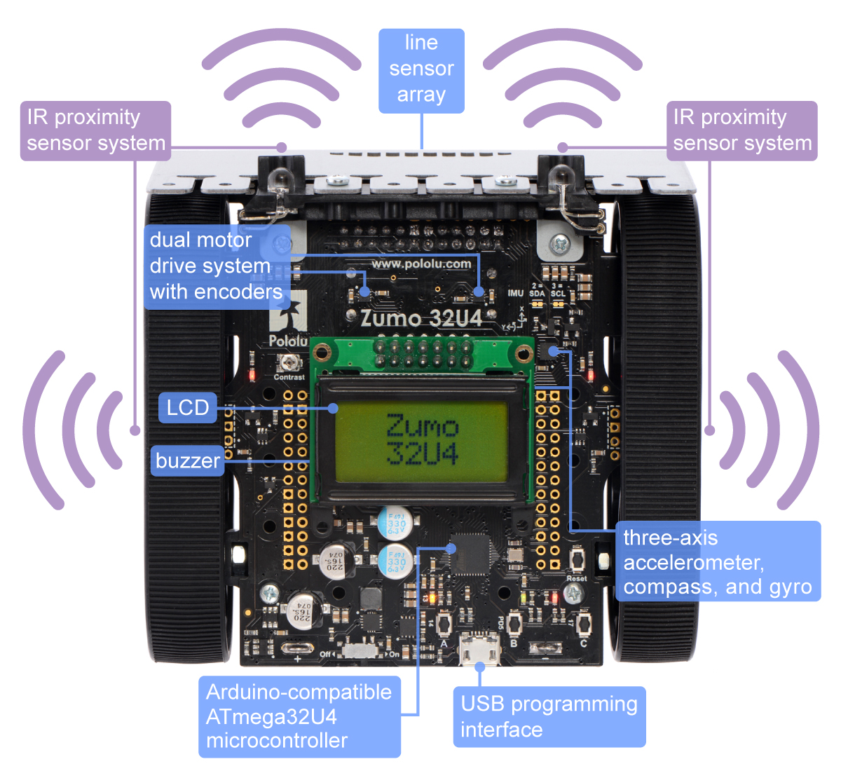
https://a.pololu-files.com/picture/0J6721.1200.jpg?f23bb5e39014c5721350a43b8c0e8fe4

Zumo32u4 Robot [1]

For the Segway implementation the Zumo32u4’s blades, line sensor array and top most IR Proximity sensors were removed because the Zumo32u4 balances on the edge where the blade is (top edge in Fig. 1). The opposite edge can’t be used because the battery (not visible in the Fig. 1) holder completely sits on the floor.

At the time of writing this documentation there are three different Zumo32u4 robots;

Zumo32u4 robot with 50:1 HP motors
Zumo32u4 robot with 75:1 HP motors
Zumo32u4 robot with 100:1 HP motors

The main difference between the available configurations is the gear ration of the motors. For this project the Zumo32u4 robot with 100:1 HP motors was used.

In the following subsections the relevant Zumo32u4 components will be described in more detail.

Inertial Management Unit¶

The Zumo32U4 includes on-board inertial sensors that can be used in advanced applications, such as helping our Zumo detect collisions and determine its own orientation by implementing an inertial measurement unit (IMU).

Note

We used IMU as the main sensory-model for Segway.

We took the aid of following sensor components of IMU;

Gyroscope : ST L3GD20H 3-axis gyroscope.
Accelerometer : ST LSM303D compass module, which combines a 3-axis accelerometer and 3-axis magnetometer.

Note

Both sensor chips share an $I^2C$ bus connected to the ATmega32U4’s $I^2C$ interface.
Level shifters built into the main board allow the inertial sensors, which operate at 3.3 V, to be connected to the ATmega32U4 (operating at 5 V).

Gyroscope¶

We consider the following aspects of Gyroscope for IMU sensory-model;

Gyroscope provides the change in orientation of the Zumo (Roll, Yaw, Pitch). Integration of result provides the position details.
ST L3GD20H Gyroscope operation is based on angular momentum.
ST L3GD20H provides; * Selectable full-scale range of $\pm245dps$/$\pm500dps$/

$\pm2000dps$, with the $8.75\frac{mdps}{digit}$/ $17.5\frac{mdps}{digit}$/$70\frac{mdps}{digit}$ sensitivity, respectively.
- Selectable data sampling rate.
- Low-Pass filter to reduce noise with selectable cut-off frequencies.

Gyroscope configuration [9]¶

// Set up the L3GD20H gyro.
gyro.init();

// 800 Hz output data rate,
// low-pass filter cutoff 100 Hz.
gyro.writeReg(L3G::CTRL1, 0b11111010);

// 2000 dps full scale.
gyro.writeReg(L3G::CTRL4, 0b00100000);

// High-pass filter disabled.
gyro.writeReg(L3G::CTRL5, 0b00000000);

Note

All other register were left with their default value. Review [13] for more information regarding default values.

A more detailed descriptions of the configuration used is shown below;

L3G::CTRL1.DR[1:0] = 0x3 selects the $800 Hz$ data sampling rate [13].

L3G::CTRL1.BW[1:0] = 0x3 selects $100 Hz$ gyroscope data cut-off frequency [13].

L3G::CTRL1.PD = 0x1 selects the normal mode disabling power mode, so the signal will be always be sampled [13].

L3G::CTRL1.XEN = 0x0, L3G::CTRL1.YEN = 0x1 and L3G::CTRL1.ZEN = 0x0 enables only the needed gyroscope channel.

L3G::CTRL4.FS[1:0] = 0x2 selects the full-scale of $\pm2000dps$ with a sensitivity of $70mdps/digit$ [13].

L3G::CTRL5.HPen = 0x0 disable the High-Pass filter [13].

Accelerometer¶

We consider the following aspects of Accelerometer for IMU sensory-model;

ST LSM303D Accelerometer provides the linear acceleration based on vibration.
By virtue of linear acceleration, Accelerometer provides 3-dimensional position (X-,Y-,Z- axis). [14]
ST LSM303D provides $\pm2$/$\pm4$/$\pm6$/$\pm8$/ $\pm16$ selectable linear acceleration full-scale. [14]
ST LSM303D provides $3.125Hz$/$6.25Hz$/$12.5Hz$/ $25Hz$/$50Hz$/$100Hz$/$200Hz$/$400Hz$/ $800Hz$/$1600Hz$ selectable sampling rate. [14]

For the implementation of the Segway the sampling frequency, $f_s = 50Hz$, and full-scale range, $acc_{range} = \pm8g$, were selected. Therefore, the ST LSM303D configuration code is shown in Listing 2

Compass configuration [9]¶

// Set up the LSM303D accelerometer.
compass.init();

// 50 Hz output data rate
compass.writeReg(LSM303::CTRL1, 0x57);

// 8 g full-scale
compass.writeReg(LSM303::CTRL2, 0x18);

Note

All other register were left with their default value. Review [14] for more information regarding default values.

A more detailed descriptions of the configuration used is shown below;

LSM303::CTRL1.AODR[3:0] = 0x5 sets the $f_s = 50Hz$. [14]

LSM303::CTRL1.BDU = 0x1 enables atomic update for the acceleration read register. Meaning that the entire register will be written at once [14].

LSM303::CTRL1.AXEN = 0x1, LSM303::CTRL1.AYEN = 0x1 and LSM303::CTRL1.AZEN = 0x1 enables all three acceleration channels. [14]. All three are needed because the magnitude of the acceleration vector is calculated to filter some measurement noise. Listing 4 shows how the magnitude is used to filter the noise.

LSM303::CTRL2.AFS[2:0] = 0x3 sets $acc_{range} = \pm8g$.

Combine Gyroscope and Accelerometer¶

Gyroscope gives angular position but has tendency to drift over the period of time. Accelerometer gives Inertia, and ultimately position but it is slow. Hence, Accelerometer output is used to correct position obtained from Gyroscope on periodic interval of time.

First the Gyroscope is being sampled as frequently as possible. Then the data of the Gyroscope is integrated and to give the current Zumo32u4’s angle as fast as possible. Listing 3 shows how the sampling and integration was performed;

Gyroscope angle sampling and integration [9]¶

/** Zumos Gyro */
L3G gyro;


/**
* Reads the Gyro changing rate and integrate it adding it to the angle
*/
void sampleGyro() {
  // Figure out how much time has passed since the last update.
  static uint16_t lastUpdate = 0;
  uint16_t m = micros();
  uint16_t dt = m - lastUpdate;
  float gyroAngularSpeed = 0;
  lastUpdate = m;

  gyro.read();
  // Obtain the angular speed out of the gyro. The gyro's
  // sensitivity is 0.07 dps per digit.
  gyroAngularSpeed = ((float)gyroOffsetY - (float)gyro.g.y) * 70 / 1000.0;

  // Calculate how much the angle has changed, in degrees, and
  // add it to our estimation of the current angle.
  angularPosition += gyroAngularSpeed * dt / 1000000.0;
}

The selected sampling frequency for all sensors was $f_s=50Hz$ meaning that every $20ms$ the integrated angle from the gyroscope is corrected with the angle given by the Accelerometer. Listing 4 shows how the correction is performed.

Integrated gyroscope angle correction with accelerometer’s angle [9]¶

/** Zumos Accelerometer */
LSM303 compass;


/**
 * Read the acceleormeter and adjust the angle
 */
void sampleAccelerometer() {
  static uint16_t lastUpdate = 0;
  uint16_t m = micros();
  uint16_t dt = m - lastUpdate;
  float gyroAngularSpeed = 0;

  lastUpdate = m;

  compass.read();
  accelerometerAngle = atan2(compass.a.z, -compass.a.x) * 180 / M_PI;

  // Calculate the magnitude of the measured acceleration vector,
  // in units of g.
  LSM303::vector<float> const aInG = {
    (float)compass.a.x / 4096,
    (float)compass.a.y / 4096,
    (float)compass.a.z / 4096}
  ;
  float mag = sqrt(LSM303::vector_dot(&aInG, &aInG));

  // Calculate how much weight we should give to the
  // accelerometer reading.  When the magnitude is not close to
  // 1 g, we trust it less because it is being influenced by
  // non-gravity accelerations, so we give it a lower weight.
  float weight = 1 - 5 * abs(1 - mag);
  weight = constrain(weight, 0, 1);
  weight /= 10;


  // Adjust the angle estimation.  The higher the weight, the
  // more the angle gets adjusted.
  angularPosition = weight * accelerometerAngle + (1 - weight) * angularPosition;
  angularSpeed = (angularPosition - prevAngularPosition) * 1000000.0 / dt;
  prevAngularPosition = angularPosition;

}

Note

Note that angularPosition is derivated to get angularSpeed, because both quantities are needed by the state variable model used. For more information review the State Variable Model.
The sign of the angle has been changed from the one in the original balancing example [9] to match our reference framework.
src/SegwayLQR/ZumoIMU.ino holds the source code that handles the IMU.

Warning

All angles are given in degrees because during implementation it was proved that it was easier to catch bugs if the angle was in degrees. One reason for this was that degrees are scaled up with respect with radians it was easier to catch integer divisions causing the angle to be zero. Furthermore the use of degrees is a little more intuitive than radians.

ZumoIMU API¶

class ZumoIMU¶

float accelerometerAngle = 0¶: Accelerometer angle

L3G gyro¶: Zumo’s Gyro

LSM303 compass¶: Zumo’ss Accelerometer

float gyroOffsetY¶: Gyro’s bias

float prevAngularPosition = 0¶: Previous Angular position

void setupIMU()¶: Setup the Gyro and Accelerometer

void sampleGyro()¶: Reads the Gyro changing rate and integrate it adding it to the angle

void sampleAccelerometer()¶: Read the accelerometer and adjust the angle

void calibrateGyro()¶: Calibrate the Gyroscope. Get the bias.

[9]	(1, 2, 3, 4, 5) Pololu. Zumolibrary’s balancing example code. URL: https://github.com/pololu/zumo-32u4-arduino-library/tree/master/examples/Balancing.

[13]	(1, 2, 3, 4, 5, 6) STMicroelectronics. L3GD20H, MEMS motion sensor: three-axis digital output gyroscope. June 2012. URL: https://www.pololu.com/file/0J731/L3GD20H.pdf.

[14]	(1, 2, 3, 4, 5, 6, 7) STMicroelectronics. LSM303D, Ultra compact high performance e-Compass 3D accelerometer and 3D magnetometer module. June 2012. URL: https://www.pololu.com/file/0J703/LSM303D.pdf.

Motors¶

The Zumo32U4 includes a DRV8837 [2] as a dual motor driver. The DRV8837 handles the current requirements for motors. It also provides rotational direction control of the motors.

The Zumo Library [8] provides the following API to control the motors’ speed.

class Zumo32U4Motors¶

Controls motor speed and direction on the Zumo 32U4.

void setSpeeds(int16_t leftSpeed, int16_t rightSpeed)¶

Sets the speeds for both motors.

int16_t leftSpeed: A number from -400 to 400 representing the speed and direction of the left motor. Values of -400 or less result in full speed reverse, and values of 400 or more result in full speed forward.

int16_t rightSpeed: A number from -400 to 400 representing the speed and direction of the right motor. Values of -400 or less result in full speed reverse, and values of 400 or more result in full speed forward.

Zumo32U4Motors::setSpeeds() enables us to control both motors. For instance a $400$ value in leftSpeed will set the a 100% duty cycle with level $6V$ PWM between the left motor’s DRV8837’s outputs (OUT1 and OUT2). Which results in applying full forward speed to the left motor. A value of $-200$ will set a 50% duty cycle with level of $-6V$ PWM between the left motor’s DRV8837’s outputs (OUT1 and OUT2).

The PWM duty cycle can be translated into a percentage of maximum current applied to the motor $I_{max}$. Table 1’s shows the value of $I_{max}$ which corresponds to the Stall Current at 6V. Additionally, the torque of the motor is linearly related to the current is applied to it. Therefore, the torque of the motors can be calculated by;

\[\tau_0 = \frac{\tau_s}{400} \times speed_{PWM}\]

Where $\tau_s$ is the stall torque of the motor at 6V. In our case we used $\tau_t = 0.211846 Nm$.

Motors’ Torque related information per Zumo32u4 model [11]¶
Model	Stall Torque @ 6V ($Nm$)	Free-run Speed @ 6V ($RPM$)	Stall Current @ 6V ($A$)
75:1	$0.105923$	$625$	$1.6$
50:1	$0.155354$	$400$	$1.6$
100:1	$0.211846$	$320$	$1.6$

[2]	Texas Instruments. Texas Instruments DRV8837/DRV8838 motor driver datasheet. June 2012. URL: https://www.pololu.com/file/0J806/drv8838.pdf.

[8]	Pololu. Zumo library. URL: https://github.com/pololu/zumo-32u4-arduino-library.

[11]	Pololu. Zumo 32u4 robot (assembled with 100:1 hp motors). 2017. URL: https://www.pololu.com/product/3127.

Encoders¶

The Zumo32U4 includes on-board encoders for closed-loop motor control. In our application we need to read the angular position and angular speed of the motors because to the Segway model we used defines these quantities as state variables. For more information review the State Variable Model.

The optical encoder [7] available in the Zumo32u4 uses the Sharp GP2S60 [12]. In the case of the encoders the Zumo Library [8] abstracts all the needed configuration and read/write operations. The only thing needed for implementation is the interpretation of the count provided by the encounters.

According to [7] the optical encoder provides 12 CPR. Therefore its count can be interpreted as shown in (1).

()¶\[cycles = \frac{encodersCount}{12 \times gearRatio}\]

According to [5], [6] and [4] the gear ratio for the different Zumo modules are shown in Table 2.

Gear Ratio and Count to Degree per Zumo32u4 model¶
Model	Gear Ratio	Count to Degree ($^\circ$)
50:1	51.45	$0.58309^\circ$
75:1	75.81	$0.39573^\circ$
100:1	100.37	$0.29889^\circ$

Furthermore we can convert number of cycles to degree with the conversion ratio $\frac{360^\circ}{1 \times cycle}$. Multiplying (1) by this ratio;

\[motorAngularPosition = encodersCount \times countToDegrees\]

With;

\[countToDegrees = \frac{360}{12 \times gearRatio}\]

Note

Since the Zumo32u4 has one encoder per motor we decided to estimate the actual motor:motorAngularPosition as the average of both motors’ angular position.

Listing 5 shows the implementation of the explained above. Note that the $motorAngularSpeed$ is obtained by derivating $motorAngularPosition$ both are needed by our state variable model. For more information review the State Variable Model.

Encoders Code¶

/** Zumo 100:1 motor gear ratio */
const float gearRatio = 100.37;
/** Encoder count to cycle convertion constant */
const float countToDegrees = 360 / (float)(12.0 * gearRatio);

/** Zumo encoders */
Zumo32U4Encoders encoders;

/**
* Clear the counters of the encoder
*/
void clearEncoders() {
  encoders.getCountsAndResetLeft();
  encoders.getCountsAndResetRight();
}

/**
* Sample the encoders
*/
void sampleEncoders() {
  static float prevPosition = 0;
  static uint16_t lastUpdate = 0;
  static float leftPosition = 0;
  static float rightPosition = 0;
  uint16_t m = micros();
  uint16_t dt = m - lastUpdate;
  lastUpdate = m;

  leftPosition += (float)encoders.getCountsAndResetLeft() * countToDegrees;
  rightPosition += (float)encoders.getCountsAndResetRight() * countToDegrees;
  float motorAngularPosition = -(leftPosition + rightPosition) / 2.0;

  motorAngularSpeed = (motorAngularPosition - prevPosition) * 1000000.0 / dt;
  prevPosition = motorAngularPosition;
}

Note

encoders.getCountsAndResetLeft() and encoders.getCountsAndResetRight() get the actual count of the respective motor and clear its counter.
$motorAngularPosition$ is the average of both speeds multiplied by $-1$ to match our reference frame.
The source code of the Encoders can be reviewed at src/SegwayLQR/ZumoEncoders.ino

ZumoEncoders API¶

class ZumoEncoders¶

const float gearRatio = 100.37¶: Zumo 100:1 motor gear ratio

const float countToDegrees = 360 / (float)(12.0 * gearRatio);: Encoder count to cycle convertion constant

Zumo32U4Encoders encoders¶: Zumo encoders

void clearEncoders()¶: Clear the counters of the encoder

void sampleEncoders()¶: Sample the encoders

[4]	Pololu. 100:1 micro metal gearmotor hp 6v with extended motor shaft. URL: https://www.pololu.com/product/2214.

[5]	Pololu. 50:1 micro metal gearmotor hp 6v with extended motor shaft. URL: https://www.pololu.com/product/2213.

[6]	Pololu. 75:1 micro metal gearmotor hp 6v with extended motor shaft. URL: https://www.pololu.com/product/2215.

[7]	(1, 2) Pololu. Optical encoder pair kit for micro metal gearmotors. URL: https://www.pololu.com/product/2590.

[8]	Pololu. Zumo library. URL: https://github.com/pololu/zumo-32u4-arduino-library.

[12]	Sharp. GP2S60, SMT, Detecting Distance : 0.5mm, Phototransistor Output, Compact Reflective Photointerrupter. October 2005. URL: https://www.pololu.com/file/0J683/GP2S60_DS.pdf.

[1]	(1, 2) Pololu. Zumo 32u4 robot. 2017. URL: https://www.pololu.com/category/170/zumo-32u4-robot.

Segway Model¶

The model of the balancing robot proposed in [15] is derived from the physical description of Fig. 2.

Segway’s relevant parameters [15]

Where;

$x$ is the horizontal position of the center of the wheel.
$\varphi$ is the clockwise rotation angle of the wheel from the horizontal axis
$\theta$ is the clockwise rotation angle of the Zumo32u4 from the horizontal axis
$m$ is the mass of the entire robot
$m_w$ is the mass of the wheel
$R$ radius of the wheel
$L$ length between the center of the wheel and the COM
$\tau_0$ is the applied torque
$I$ inertia of the body part
$I_w$ inertia of the wheel

System’s dynamics equations¶

The obtained differential equations of the system in [15] are;

()¶\[\begin{split}E \begin{bmatrix} \ddot{\varphi} \\ \ddot{\theta} \end{bmatrix} \ \ + F \begin{bmatrix} \dot{\varphi} \\ \dot{\theta} \end{bmatrix} \ \ + G \theta = H\tau_0\end{split}\]

With,

\[\begin{split}E = \begin{bmatrix} I_w + (m_w + m)R^2 & mRL \\ mRL & I + mL^2 \end{bmatrix}\end{split}\]

\[\begin{split}F = \begin{bmatrix} \beta_\gamma + \beta_m & -\beta_m \\ -\beta_m & \beta_m \end{bmatrix}\end{split}\]

\[\begin{split}G = \begin{bmatrix} 0 \\ -mgL \end{bmatrix}\end{split}\]

\[\begin{split}H = \begin{bmatrix} 1 \\ -1 \end{bmatrix}\end{split}\]

Model Adaptation¶

In [15] they define $L$ as in (3) with the variables define as in Fig. 3.

()¶\[L = \frac{L_2}{2} + \frac{L_1 + L_2}{2}\frac{m_1}{m}\]

Center of Mass calculation [15]

Similarly [15] defines the inertia momentum of the robot as in (4).

()¶\[I = m_1(\frac{L_1}{2}+L_2)^2 \frac{1}{12}m_2L_2^2\]

Given the geometry of the Zumo32u4 we consider that $m_1 = 0$ and $L_1 = 0$. Therefore the distance to the COM and the inertia momentum can be calculated $L = \frac{L_2}{2}$ and $I = \frac{1}{12}m_2L_2^2$, respectively.

Furthermore, the model in [15] consider a normal wheel. In our Zumo32u4 we have a caterpillar system. (5) shows how the inertia moment of the caterpillar system was calculated.

()¶\[I_w = I_{w_1} + I_c + I_{w_2}\]

Where the $I_{w_1}$ and $I_{w_2}$ are the inertia moment of the both wheels and $I_c$ is the inertia moment of the caterpillar band. In our case both wheels are equal and can be calculated as in (6)

()¶\[I_{w_i} = m_wR^2\]

Additionally the inertia of the caterpillar band can be calculated as shown in (7). Where $m_c$ is the mass of the caterpillar band.

()¶\[I_c = m_cR^2\]

Finally the inertia moment of the entire caterpillar system can be calculated as in (8).

()¶\[I_w = (2\cdot m_w + m_c)R^2\]

Input Adaptation¶

The model in [15] defines the input to be the torque $\tau_0$. Since the actual input to our system is the PWM applied to the motors we can use the equation defined in the subsection Motors of the chapter Zumo32u4, shown in (9).

()¶\[\tau_0 = \frac{\tau_s}{400} \times speed_{PWM}\]

Merging (9) and (2) we obtain;

\[\begin{split}E \begin{bmatrix} \ddot{\varphi} \\ \ddot{\theta} \end{bmatrix} \ \ + F \begin{bmatrix} \dot{\varphi} \\ \dot{\theta} \end{bmatrix} \ \ + G \theta = H_1speed_{PWM}\end{split}\]

With;

\[H_1 = H * \frac{\tau_s}{400}\]

State Variable Model¶

Finally the state variable model of the system can be calculated as shown in (10).

()¶\[ \begin{align}\begin{aligned}\dot{x} = Ax + Bu\\y = Cx + D\end{aligned}\end{align} \]

With the state variable vector;

\[\begin{split}x = \begin{bmatrix} \varphi \\ \theta \\ \dot{\varphi} \\ \dot{\theta} \end{bmatrix}\end{split}\]

And the constant matrices;

\[\begin{split}A = \left[ \begin{array}{c|c|cc} \begin{matrix} 0 \\ 0 \end{matrix} & \begin{matrix} 0 \\ 0 \end{matrix} & \begin{matrix} 1 & 0 \\ 0 & 1 \end{matrix} \\ \hline \begin{matrix} 0 \\ 0 \end{matrix} & -E^{-1}G & -E^{-1}F \end{array} \right]\end{split}\]

\[\begin{split}B = \left[ \begin{array}{c} \begin{matrix} 0 \\ 0 \end{matrix} \\ \hline -E^{-1}H \end{array} \right]\end{split}\]

\[\begin{split}C = \begin{bmatrix} 1 & 0 & 0 & 0 \\ 0 & 1 & 0 & 0 \\ 0 & 0 & 1 & 0 \\ 0 & 0 & 0 & 1 \end{bmatrix}\end{split}\]

\[\begin{split}D = \begin{bmatrix} 0 \\ 0 \\ 0 \\ 0 \end{bmatrix}\end{split}\]

[15]	(1, 2, 3, 4, 5, 6, 7, 8) Mie Kunio Ye Ding, Joshua Gafford. Modeling, simulation and fabrication of a balancing robot. Technical Report, Harvard University, Massachusettes Institute of Technology, 2012.

LQR Controller Design¶

The controller to be implemented is a full-state feedback controller. The LQR controller was selected. Fig. 4 shows the block diagram of the entire system to be implemented.

$digraph { graph [rankdir=LR, splines=ortho, concentrate=true]; node [shape=polygon]; node[group=main]; System [ label="Segway \n ẋ = Ax(t) + Bu(t)", rank=1]; i [shape=point]; x [shape=plaintext, label=""]; C [ label="C" ]; y [shape=plaintext, label=""]; System -> i [ dir="none", label="x(t)" ]; i -> C; C -> y [ label="y(t)"]; node[group="feedback"]; Feedback [ label="-K", rank=1 ]; Feedback -> System [ label="u(t)"]; Feedback -> i [ dir=back ]; }$

Full-state feedback block diagram¶

Physical parameters¶

All the parameters needed for the model can be seen in Listing 6

Physical constant script scripts/load_physical_constants.m [1]¶

% Sampling constants
T_s = 20e-3;
f_s = 1/T_s;

% Constants (context)
m = 0.24200; % Mass of the zumo
m_1 = 0;
m_2 = m;
L_1 = 0;
L_2 = 0.062;
L = L_2/2 + (L_1 + L_2) * m_1/(2*m); % Height of the zumo
beta_m = 0.01;
beta_gamma = 0.01;

g =  9.8100; % Gravitational constant
R = 0.019; % Wheel radius

I = m_1*(L_1/2 + L_2)^2 + (m_2*L_2^2)/12; % Inertial momentum

m_w = 0.004; % Mass of the wheel
m_c = 0.009; % Mass of the caterpillar band

I_w_i = m_w*R^2; % Inertia momentum of wheels
I_c = m_c*R^2; % Inertia momentum of Caterpillar band
I_w = 2*I_w_i + I_c; % Inertia momentum of Caterpillar system

% Motor's constants
motor_stall_torque = 0.211846554999999; % According to specs 30 oz-in
pulse2torque = motor_stall_torque/400;

Note

For $\beta_m$ and $\beta_\gamma$ are set to a dummy value as in [15].

Model¶

To setup the model the script in Listing 7 was used.

Get State Variable Model script scripts/get_ssmodel.m [1]¶

function model = get_ssmodel()

  % Consants (context)
  load_physical_constants

  E = [(I_w + (m_w + m)*R^2) m*R*L;
       m*R*L (I + m*L^2)];

  F = [(beta_gamma + beta_m) -beta_m;
       -beta_m beta_m];

  G = [0; -m*g*L];

  H_1 = [1; -1] * pulse2torque;

  states = size(E, 1);

  A = [zeros(states) eye(states);
       zeros(states, 1) -inv(E)*G -inv(E)*F];
  B = [zeros(states, 1);
       -inv(E)*H_1];
  C = [1 0 0 0;
       0 1 0 0;
       0 0 1 0;
       0 0 0 1];
  D = [0; 0; 0; 0];

  model = ss(A, B, C, D);

end

A second script, shown in Listing 8 was also added to get the model that also obtains the transfer function $H(s) = \frac{\Theta(s)}{S(s)}$. Where, $S(s)$ is the Laplace transform of the $speed_{PWM}$ function. This transfer function was used to further analysis not presented in this documentation.

Get Model script scripts/get_model.m [1]¶

function [plant, model] = get_model()

  % Get the state variable model
  model = get_ssmodel();

  % Get the transfer function
  plant = tf(model);
  plant = plant(2);

end

Controllability¶

Before the actually designing the controller we need to check it’s controllability. The controllability check done can be seen in Listing 9.

Check controllability scripts/lqr_design.m [1]¶

% Check controlability
co =  ctrb(model);
if (rank(co) > n_states)
  disp(" -> Error! System isn't controllable");
  return;
else
  disp(" -> Great! System is controllable");
end

Observability¶

Similarly, the system’s observability has to be also verified. This verification is shown in Listing 10.

Check Observability scripts/lqr_design.m [1]¶

ob = obsv(model);
if (rank(ob) > n_states)
  disp(" -> Error! System isn't observable");
  return;
else
  disp(" -> Great! System is observable");
end

Control Law¶

To obtain the control law $K$ the script in Listing 11.

Control Law Calculation scripts/lqr_design.m [1]¶

Q = eye(size(model.a,1));

R = 1

[K, X, P] = lqr(model, Q, R);

K_s = K*pi/180;

Note

As in [15] equally weighted states and outputs were used. Therefore, $Q = I$ and $R = 1$. Where, $I$ is an identity matrix with the size of $A$.
A scaled control law $K_s$ is also calculated. The scale factor is needed because the angles measured by accelerometer/gyro and encoders was done in degrees.

The obtained control law is shown in (11). And the scaled version in (12)

()¶\[K = \begin{bmatrix} 1 & 483.6133 & 10.0038 & 20.3053 \end{bmatrix}\]

()¶\[K_s = \begin{bmatrix} 0.0175 & 8.4406 & 0.1746 & 0.3544 \end{bmatrix}\]

Controller Simulation¶

After designing the control law the controller is simulated as shown in Listing 12.

Controller simulation excerpt scripts/lqr_design.m [1]¶

Ac = model.a - model.b*K;
sys_cl = ss(Ac, model.b, model.c, model.d);
figure(1);
clf(1)
impulse(sys_cl);

The simulation results can be seen in Fig. 5. Since the $\frac{d\varphi}{dt}$ and $\frac{d\theta}{dt}$ are faster variables a zoomed result simulation result can also be seen in Fig. 6.

LQR Design Simulation Results

LQR Design Zoomed Simulation Results

Further Features¶

Arduino Pretty Printing¶

For rapid deployment and testing the scripts/lqr_design.m also prints the scaled control law in the Arduino language. An example output can be seen in Listing 14 and the script excerpt that implement this functionality in Listing 13.

Arduino Code control law generator scripts/lqr_design.m [1]¶

disp("Control Law")
K_string = strcat("const float K[", num2str(size(model.a,1)), "] = {");
for k = 1:size(K, 2)
  if ~(k == 1)
    K_string = strcat(K_string, ", ");
  end
  K_string = strcat(K_string, num2str(K_s(k)));
end
K_string = strcat(K_string, "};");
disp("K")
disp(K_string)

Arduino Code control law generator output¶

Control Law
K
const float K[4] = {0.017453, 8.4406, 0.1746, 0.35439}

Closed-Loop Poles¶

scripts/lqr_design.m also print out the closed-loop poles. An example output can be seen in Listing 15.

Closed-loop printing output example¶

P =

 1.0e+03 *

 -1.0872
 -0.0000
 -0.0083
 -0.0178

Full-compensator design¶

In scripts/lqr_design.m the full compensator design flow is implemented but since it’s not being implements it’s was left out of this documentation.

[1]	(1, 2, 3, 4, 5, 6, 7, 8) Pedro Cuadra Meghadoot Gardi. Pjcuadra/zumogetway. August 2017. URL: https://github.com/pjcuadra/zumosegway.

[15]	(1, 2) Mie Kunio Ye Ding, Joshua Gafford. Modeling, simulation and fabrication of a balancing robot. Technical Report, Harvard University, Massachusettes Institute of Technology, 2012.

Controller Implementation¶

The implementation of the controller system was done using Arduino IDE. The functionality was separated into files within the Arduino IDE project. ZumoIMU and ZumoEncoders files where already explained in the sections Inertial Management Unit and Encoders.

SegwayLQR¶

SegwayLQR API¶

Global Constants¶

const uint8_t samplingPeriodMS = 20¶: Sampling Period in ms

const float samplingPeriod = samplingPeriodMS / 1000.0;: Sampling Period in s

const float samplingFrequency = 1 / samplingPeriod¶: Sampling frequency

const uint8_t statesNumber = 4¶: Number states

Global Variables¶

float angularPositionLP = 0¶: Low pass filter angular Position

float angularPosition = 0¶: Zumo’s angular position

float correctedAngularPosition = 0¶: Corrected angular position

float angularSpeed = 0¶: Zumo’s angular speed

float motorAngularPosition = 0¶: Motor’s angular position

float motorAngularSpeed = 0¶: Motor’s angular speed

int32_t speed¶: PWM signal applied to the motor’s driver 400 is 100% cycle and -400 is 100% but inverse direction

Zumo32U4ButtonA buttonA¶: A button of the zumo board

Zumo32U4Motors motors¶: Zumo robot’s motors

Functions¶

class SegwayLQR¶

void setup()¶: Segway’s setup function.

void loop()¶: Segway’s loop function.

void setActuators()¶: Set the values to the actuators.

SegwayLQR Details¶

src/SegwayLQR/SegwayLQR.ino features the main loop and setup functions of the Arduino project. Listing 16 shows the implementation of the setup function. Firstly, it setups the IMU by calling ZumoIMU::setupIMU(). Then, calibrates the IMU’s gyro by calling ZumoIMU::calibrateGyro(). After calibrating it starts a loop of sampling the gyro as frequently as possible and the accelerometer every samplingPeriod. When the buttonA is pressed the loop is exited and before starts executing SegwayLQR::loop() the encoders counters are cleared by calling ZumoEncoders::clearEncoders().

Setup function¶

/**
 * Setup Function
 */
void setup() {
  Wire.begin();

  Serial.begin(115200);

  // Setup the IMU
  setupIMU();

  // Calibrate the IMU (obtain the offset)
  calibrateGyro();

  // Display the angle until the user presses A.
  while (!buttonA.getSingleDebouncedRelease()) {
    // Update the angle using the gyro as often as possible.
    sampleGyro();

    // Sample accelerometer every sampling period
    static uint8_t lastCorrectionTime = 0;
    uint8_t m = millis();
    if ((uint8_t)(m - lastCorrectionTime) >= samplingPeriodMS)
    {
      lastCorrectionTime = m;
      sampleAccelerometer();
    }
  }
  delay(500);
  clearEncoders();
}

Listing 17 shows the loop function’s code. Basically does the same as in the loop in SegwayLQR::setup() but every samplingPeriod it;

ZumoIMU::sampleAccelerometer() to obtain the corrected estimation of the Zumo’s angle and angular speed, as explained in Inertial Management Unit.
ZumoEncoders::sampleEncoders() to obtain encoders position and speed, as explained in Encoders.
SegwayLQR::setActuators() calculates the new speed to be set based on the current state variables’ state and the LQR designed control law.

Loop function¶

/**
 * Main loop Function
 */
void loop() {
  // Update the angle using the gyro as often as possible.
  sampleGyro();

  // Every 20 ms (50 Hz), correct the angle using the
  // accelerometer, print it, and set the motor speeds.
  static byte lastCorrectionTime = 0;
  byte m = millis();
  if ((byte)(m - lastCorrectionTime) >= 20)
  {
    lastCorrectionTime = m;
    sampleAccelerometer();
    sampleEncoders();
    setActuators();
  }
}

Listing 18 shows the SegwayLQR::setActuators() function’s code. As a security measure when the angle is greater that $45^\circ$ the speed is set to zero. Furthermore, the angle is corrected by the deviation of the COM from the actual horizontal center of the Zumo32u4. Finally the LQR::lqr() is called to apply the control law and generate the input of the system.

Set actuators function¶

/**
 * Control the actuators
 */
void setActuators() {
  const float targetAngle = 1.45;

  if (abs(angularPosition) > 45) {
    // If the robot is tilted more than 45 degrees, it is
    // probably going to fall over.  Stop the motors to prevent
    // it from running away.
    speed = 0;
  } else {
    correctedAngularPosition = angularPosition - targetAngle;
    lqr();
    speed = constrain(speed, -400, 400);
  }

  motors.setSpeeds(speed, speed);
}

LQR¶

LQR API¶

class LQR¶

const float K[statesNumber] = {0.55192, 8.9867, 0.194, 0.39237}¶: Control Law

const float scaleConst = 2.5¶: Correction factor gain factor

void lqr()¶: Apply LQR control law

LQR Details¶

Listing 19 shows how the LQR::lqr() is implemented.

Apply LQR designed control law¶

/**
 * LQR control law
 */
void lqr() {
  speed = 0;

  speed -= motorAngularPosition * K[0];
  speed -= correctedAngularPosition * K[1];
  speed -= motorAngularSpeed * K[2];
  speed -= angularSpeed * K[3];

  speed = speed*scaleConst;

}

Note

The K values are multiplied by $-1$ in according to Fig. 4.
An additional scale factor, $scaleConst = 2.5$, is introduce to compensate;
- Possible deviation of the actual Stall Torque with load.
- Bad estimation of the $\beta_m$ and $\beta_\gamma$ values.

Model	Stall Torque @ 6V (\(Nm\))	Free-run Speed @ 6V (\(RPM\))	Stall Current @ 6V (\(A\))
75:1	\(0.105923\)	\(625\)	\(1.6\)
50:1	\(0.155354\)	\(400\)	\(1.6\)
100:1	\(0.211846\)	\(320\)	\(1.6\)