Welcome to SHARPpy’s documentation!

SHARPpy is a collection of open source sounding and hodograph analysis routines, a sounding plotting package, and an interactive, cross-platform application for analyzing real-time soundings all written in Python. It was developed to provide the atmospheric science community a free and consistent source of sounding analysis routines. SHARPpy is constantly updated and vetted by professional meteorologists and climatologists within the scientific community to help maintain a standard source of sounding routines.

License

Copyright (c) 2011, Patrick T. Marsh & John Hart. All rights reserved.

Copyright (c) 2012, MetPy Developers. All rights reserved.

Copyright (c) 2018, K. T. Halbert, W. G. Blumberg, & T. A. Supinie All rights reserved.

Redistribution and use in source and binary forms, with or without modification, are permitted provided that the following conditions are met:

• Redistributions of source code must retain the above copyright notice, this list of conditions and the following disclaimer.
• Redistributions in binary form must reproduce the above copyright notice, this list of conditions and the following disclaimer in the documentation and/or other materials provided with the distribution.
• Neither the name of the MetPy Developers nor the names of any contributors may be used to endorse or promote products derived from this software without specific prior written permission.

THIS SOFTWARE IS PROVIDED BY THE COPYRIGHT HOLDERS AND CONTRIBUTORS “AS IS” AND ANY EXPRESS OR IMPLIED WARRANTIES, INCLUDING, BUT NOT LIMITED TO, THE IMPLIED WARRANTIES OF MERCHANTABILITY AND FITNESS FOR A PARTICULAR PURPOSE ARE DISCLAIMED. IN NO EVENT SHALL THE COPYRIGHT OWNER OR CONTRIBUTORS BE LIABLE FOR ANY DIRECT, INDIRECT, INCIDENTAL, SPECIAL, EXEMPLARY, OR CONSEQUENTIAL DAMAGES (INCLUDING, BUT NOT LIMITED TO, PROCUREMENT OF SUBSTITUTE GOODS OR SERVICES; LOSS OF USE, DATA, OR PROFITS; OR BUSINESS INTERRUPTION) HOWEVER CAUSED AND ON ANY THEORY OF LIABILITY, WHETHER IN CONTRACT, STRICT LIABILITY, OR TORT (INCLUDING NEGLIGENCE OR OTHERWISE) ARISING IN ANY WAY OUT OF THE USE OF THIS SOFTWARE, EVEN IF ADVISED OF THE POSSIBILITY OF SUCH DAMAGE.

Installation Guide

SHARPpy can be installed in one of two forms: either a pre-compiled binary executable or by downloading the code and installing it using a separate Python interpreter. Binary executables are available for Windows 7 (32 and 64 bit), Windows 8.1 (64 bit only), and Mac OS X 10.6+ (Snow Leopard and later; 64 bit only). If you do not have one of those, then you will need to download the code.

Installing a Pre-compiled Binary

The following pre-compiled binaries are available (click to download):

[OS X (64 Bit)](https://github.com/sharppy/SHARPpy/releases/download/v1.3.0-Xenia-beta/sharppy-osx-64.zip)

[Windows 7 (32 Bit)](https://github.com/sharppy/SHARPpy/releases/download/v1.3.0-Xenia-beta/sharppy-win7-32.zip)

[Windows 7 (64 Bit)](https://github.com/sharppy/SHARPpy/releases/download/v1.3.0-Xenia-beta/sharppy-win7-64.zip)

[Windows 8.1 and Windows 10 (64 Bit)](https://github.com/sharppy/SHARPpy/releases/download/v1.3.0-Xenia-beta/sharppy-win8.1-64.zip)

Installing a pre-compiled binary should be as simple as downloading the .zip file and extracting it to the location of your choice. The zip files are named for the operating system and number of bits. Most recently-built computers (probably post-2010 or so) should have 64-bit operating systems installed. If your computer is older and you’re unsure whether it has a 32- or 64-bit operating system, you can check on Windows 7 by clicking Start, right-clicking on Computer, and selecting Properties. All recent versions of OS X (10.6 and newer) should be 64-bit.

Installing the Code from Source

SHARPpy code can be installed on Windows, Mac OS X, and Linux, as all these platforms can run Python programs. SHARPpy may run on other operating systems, but this has not been tested by the developers. Chances are if it can run Python, it can run SHARPpy. Running the SHARPpy code requires a.) the Python interpreter and b.) additional Python libraries. Although there are multiple ways to meet these requirements, we recommend you install the Python 3.6 version of the Anaconda Python distribution. SHARPpy is primarily tested using this distribution.

The Anaconda Python Distribution can be downloaded here: https://store.continuum.io/cshop/anaconda/

Additional ways to meet these requirements may include the Enthought Python Distribution, MacPorts, or Brew, but as of this moment we cannot provide support for these methods.

Required Python Packages/Libraries:

• NumPy
• PySide

Since SHARPpy requires the PySide and Numpy packages, you will need to install them. If you choose to use the Anaconda distribution, Numpy comes installed by default. PySide can be installed through the Anaconda package manager that comes with the Anaconda distribution by opening up your command line program (Terminal in Mac OS X/Linux and Command Prompt in Windows) and typing:

conda install -c conda-forge pyside=1.2.4

After installing all the required Python packages for SHARPpy, you now can install the SHARPpy package to your computer. You’ll need to download it to your computer first and open up a command line prompt. You can download it as a ZIP file (link on the right) or clone the Git respository (you will need the git program) into a directory on your computer by typing this into your command line:

git clone https://github.com/sharppy/SHARPpy.git

If you follow the route of cloning SHARPpy, you can update to the most recent SHARPpy package by typing the following within the folder you downloaded SHARPpy to:

git pull origin master

Once the package has been downloaded to your computer, use your command line to navigate into the SHARPpy directory and type this command in to install SHARPpy:

python setup.py install

After installing the package, you can run the SHARPpy GUI and interact with the SHARPpy libraries through Python scripts.

Using the Data Picker

Launching the SHARPpy program should load up the SHARPpy Sounding Picker:

The SHARPpy Sounding Picker window showing the locations where observed sounding data may be examined through the program interface.

The Picker is an interface where the metadata for sounding data sources may be examined in order to help select the sounding data the user wishes to analyze. In this window, users can select the data source (top left) which includes both observed and modeled sounding datasets. For each sounding source, a data cycle time can be selected. For observed data, this will generally be at 00 and 12 UTC. For modeled data, the data may be available at hourly or synoptic time intervals (e.g., 00, 06, 12, or 18 UTC). If point forecast soundings are desired by the user from different models (e.g., GFS), the “Select Forecast Time” list will be populated to show the model forecast times available from that model. This list can be used to load subsets of the model run data into SHARPpy for analysis.

After the data source and times are selected, the map to the right will be populated with red points indicating the sounding locations available. While the program does default to U.S. locations, the map can be reoriented by clicking and dragging the map area. Double clicking on the map will center the map to the cursor location. Other global maps (e.g., Tropics and Southern Hemisphere) can be selected from the drop down box. Should you wish to save your map view as the new default map view, you can click the “Save Map View as Default” box in the top right. Selection of a sounding data site will turn that site green on the map. Once a sounding data site is selected, you can click “Generate Profiles” to download the data and analyze it in the SHARPpy GUI.

Default Data Sources

SHARPpy links into various datasets around the web to allow the user to explore a variety of observed and modeling datasets. Links to these datasets come default with the SHARPpy package and files pointing SHARPpy to these datasets are placed in the user’s home directory underneath a directory called .sharppy/. Unless you are attempting to install additional data sources that SHARPpy can read, this folder should not be modified.

Default SHARPpy Data Sources

Name	Link	Datasets
Penn State	http://www.meteo.psu.edu/bufkit/	HRRR, GFS, NAM, 3km NAM, SREF, RAP
NOAA SPC	https://www.spc.noaa.gov/exper/soundings/	Observed U.S. Soundings
SHARP	http://sharp.weather.ou.edu/	Observed & Archived Int. Soundings

Currently, both the NOAA SPC and SHARP server datasets are able to offer world-wide observed soundings. While the SPC server is handled by the meteorologists at the Storm Prediction Center, the SHARPpy development team has been granted server space at the University of Oklahoma to generate various datastreams (e.g. international soundings). Data from the SHARP server is generated by GEMPAK binaries that merge realtime standard and significant level data accessible here. Archived soundings were downloaded from the publically available GEMPAK data archive managed by the Iowa Environmental Mesonet. Data from this archive starts on January 1st, 1946. Decoding of this dataset (and the real-time international data stream on SHARP) are performed by the GEMPAK snlist binary distributed in the NWS SOO’s BUFRgruven package.

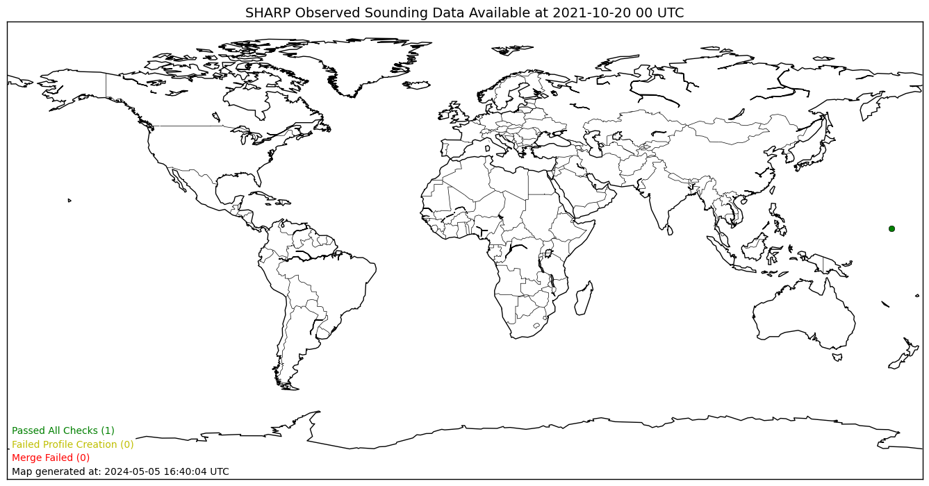
A real-time status plot from the SHARP server generated for the last (00 or 12 UTC) sounding dataset available. Each point indicates a location where sounding data was found on the Unidata stream. The color of each point indicates the status of the data in the processing steps. Green data points indicate data files that were able to be generated by the merge script and passed the SHARPpy data integrity checks. Yellow data points indicate data files that were created, but threw an exception when passed to SHARPpy (likely due to data integrity issues). Red data points are locations where the merge script failed and are likely due to incomplete data in the Unidata stream.

The data provided by Penn State is provided in the Bufkit format. The foreast soundings provided within this format are derived directly from the model native vertical grid; no interpolation is performed. Often, the forecast sounding points are located at stations where METAR observations can be found. The forecast sounding points have been chosen by the scientists at NOAA’s Environmental Modeling Center as a part of their mission to support NOAA’s mission. Although we are persuing various options for expanding the various sounding points from these models, we do not have the ability to add more data points.

Note

The SHARPpy development team has noticed a distinct sensitivity of various SHARPpy algorithms to the post-processing performed on model output. Particularly, this sensitivity is best noticed when SHARPpy output is compared between model forecast soundings a.) created by interpolated from the model vertical grid to 25-mb pressure levels and b.) those created from the native model vertical grid. Because of this sensitivity, differences may appear between different SHARPpy output across the web.

Warning

Occasionally, the default data sources go down in SHARPpy. With the exception of the SHARP dataset, these issues are largely outside of our control and may often be resolved by trying to access the data again at another time.

Changing preferences

Users may select “Preferences” using the menu bar of the SHARPpy program. Doing so will load a small window where the user can modify the SHARPpy color pallet and the units of the program. Currently, the three color pallets exist: the Standard (black background), Inverted (white background), or the Protanopia (for color blindness).

Units may be changed for the surface temperature value, the winds, and the precipitble water vapor. Switching to metric units through this method may help international users more easily use the program. These changes may be detected in the GUI, as various locations where the units are shown will switch when a new unit is selected in the Preferences.

Interpreting the GUI

Our BAMS article on SHARPpy provides an overview of the various insets and information included in the SHARPpy sounding window. Included within the paper is a list of references to journal articles which describe the relevance of each aspect of the SHARPpy sounding window to research in atmospheric science and the scientific forecasting process. This documentation provides an overview of the SHARPpy GUI features.

Additional resources for interpreting the GUI include the SPC Sounding Analysis Help and Explanation of SPC Severe Weather Parameters webpages. The first site describes the SHARP GUI, which is the basis for the SHARPpy GUI. The second can be used to help interpret some of the various convection indices shown in the SHARPpy GUI. Not all features shown on these two sites are shown in the SHARPpy GUI.

Skew-T

Various sounding variables are displayed in the Skew-T, which is a central panel of the GUI:

• Solid red – temperature profile
• Solid green – dewpoint profile
• Dashed red – virtual temperature profile.
• Cyan – wetbulb temperature profile
• Dashed white – parcel trace (e.g., MU, SFC, ML) (the parcel trace of the parcel highlighted in yellow in the Thermodynamic Inset.)
• Dashed purple – downdraft parcel trace (parcel origin height is at minimum 100-mb mean layer equivalent potenial temperature).
• Winds barbs are plotted in knots (unless switched to m/s in the preferences) and are interpolated to 50-mb intervals for visibility purposes.
• If a vertical velocity profile (omega) is found (e.g., sounding is from a model), it is plotted on the left. Blue bars indicate sinking motion, red bars rising motion. Dashed purple lines indicate the bounds of synopic scale vertical motion. Units of the vertical velocity are in microbars/second.

Note

When analyzing model forecast soundings, the omega profile can be used to determine whether or not models are “convectively contaminiated”. This means that the sounding being viewed is under the influence of convection and therefore is not representitive of the large-scale environment surrounding the storm. When omega values become much larger than synoptic scale vertical motion values, users should take care to when interpreting the data.

Parcel LCL, LFC, and EL are denoted on the right-hand side in green, yellow and purple, respectively. Levels where the environmental temperature are 0, -20, and -30 C are labeled in dark blue. The cyan and purple I-bars indicate the effective inflow layer and the layer with the maximum lapse rate between 2-6 km AGL. Information about the effective inflow layer may be found in Thompson et al. 2007.

An example of the Skew-T inset showing a model forecast sounding for May 31, 2013 at 18 UTC. The 2-6 km max lapse rate layer clearly denotes the elevated mixed layer, while the omega profile indicates that rising motion is occuring within the lowest 6 km of the sounding in the forecast.

Wind Speed Profile

The tick marks for this plot are every 20 knots (should knots be the default unit selected in the preferences).

Inferred Temperature Advection Profile

Hodograph

Although the hodograph plotted follows the traditional convention used throughout meteorology, the hodograph shown here is broken up into layers by color. In addition, several vectors are also plotted from different SHARPpy algorithms.

Bunkers Storm Motion Vectors

The storm motion vectors here are computed using the updated Bunkers et al. 2014 algorithm, which takes into account the effective inflow layer.

Corfidi Vectors

The Corfidi vectors may be used to estimate mesoscale convective system (MCS) motion. See Corfidi 2003 for more information about how these are calculated.

LCL-EL Mean Wind

Critical Angle

See Esterheld and Guiliano 2008 for more information on the use of critical angle in forecasting.

Storm Slinky

Examples

Theta-E w/ Pressure

See Atkins and Wakimoto 1991 for more information on what to look for in this inset when forecasting wet microbursts.

Storm-Relative Winds w/ Height

See Rasmussen and Straka 1998 for more information on how the anvil-level storm relative winds may be used to predict supercell morphology. See Thompson et al. 2003 for information on using the 4-6 km storm-relative winds to predict tornado environments.

Possible Hazard Type

Flowchart

SHARPpy Insets

At the bottom of the SHARPpy GUI lies four separate insets that can be used to assist in analyses of the sounding data. The two insets highlighted in yellow are interchangeable with some of the other insets provided in the program.

Thermodynamic Indices

Kinematic Indices

Provides information on the storm-relative helicity (SRH), wind shear (Shear), pressure-weighted mean wind (MnWind) and layer-averaged storm-relative winds (SRW) for different layers. Layers shown here have been shown to correspond to storm longevity, storm mode, and tornado potential. The Bunkers storm motion and Corfidi vectors are also displayed.

Sounding Analog Retrieval System (SARS)

Sounding Analogue Retrieval System to compare soundings with previous severe weather environments.

Sounding Analog Retrieval System provides matching of the current sounding to past severe weather events. Clicking on any of the close matches will load the sounding from that event into the sounding window for closer comparison and inspection (see Jewell et al.). Atempts to match the current sounding to past proximity soundings from tornado and hail events using sounding parameters. “Loose” matches are used to provide a probability of hail exceeding 2 inches and a tornado intensity exceeding EF2. The algorithm is calibrated to maximize probability of detection.

Strict (very close) matches are also displayed showing the date, time, location, and threat magnitude

• Supercells may have no tornado (NON), a weak tornado (WEAK) or a significant tornado (EF2+) (SIG).
• Hail size is indicated in the strict matches.

Sig-Tor Stats

STP Ingredients and EF Probabilties for diagnosing tornadic environment ingredients.

Information on the significant tornado parameter with CIN (STPC) associated with the sounding (see Thompson et al. 2012, WAF). Distributon of STP (effectve-layer) with tornado intensity for right-moving supercells. Whiskers indicate 10th-90th percentile values, while the box indicates the interquartile range and the median. Colored horizontal line indicates the value of STPE.

The smaller inset embedded within this one indicates the relative frequency of EF2+ tornado damage with right moving supercells for STPE and its individual components (e.g., MLLCL, MLCAPE, EBWD, ESRH). Frequency values change color (similar to the Thermodynamic inset) as the probability increases.

Sig-Hail Stats

Expected Hail Sizes based on the SHIP parameter using a hail climatology.

Distribution of expected hail sizes associated with the significant hail parameter (SHIP).

Fire Weather

Fire weather parameters and guidance.

Provides a list of variables relevant to the moisture and wind properties within the convective boundary layer. See Fosberg (1978) for information on the Fosberg Fire Weather Index (FWI). PW changes color if the MUCAPE > 50 J/kg, PW < 0.5 inches, and SFC RH is < 35 % to alert the user if the potential exists for fire starting, dry thunderstorms.

Winter Weather

• Provides information regarding the mean atmospheric properties within the Dendritic Growth Zone (DGZ; -12 ̊C to -17 ̊C layer), which is the layer where most types of ice nuclei can become activated and grow into ice crystals (e.g., snow).
• Provides an estimate of the initial precipitation phase using empirical arguments.
• Identifies layers where falling precipitation may experience melting/freezing by considering the wetbulb temperature profile and environmental temperature profile.
• Performs a best guess precipitation type using Bourgouin (2000) precipitation algorithm, the initial precipitation phase, and surface temperature.
• Uses top-down preciptation type thinking.

EF Scale Probablities (STP)

Conditional probability of meetingng or exceeding a given EF scale rating for max STP (effective-layer w/ CIN) within 80 km of a tornado (all convective mode events).

Conditional probablities for different tornado strengths based on STPC (see Smith et al. 2015, WAF). Applies only if a tornado is present.

EF Scale Probablities (VROT)

Conditional WSR-88D 0.5 Deg. Azimuthal Shear Tornado Intensity Probabilities

Conditional probabilities for different tornado strengths based on the 0.5 degree rotational velocity. (Double click inside the inset to input a VROT value…see Smith et al. 2015, WAF). The inset assesses the conditional probability of maximum tornado EF scale by combining information on the near-storm environment, the convective mode, and the 0.5 ̊ peak VROT (from WSR-88D).

Interacting with the GUI

For information on the interactive aspects of the program, see the sections below:

Zooming and Changing Views

Your mouse wheel or trackpad will allow you to zoom on both the Hodograph and Skew-T plots within the window. Right clicking on the Hodograph will also allow you to change where the hodograph is centered. Currently, the hodograph can be centered on the Right Mover Storm Motion Vector, the Cloud-Layer Mean Wind Vector, or the origin of the hodograph.

Swapping Insets

The right 2 insets of the SHARPpy program can be changed by right clicking on either one. Right clicking will bring up a menu that shows the different insets available for the user. These insets exist to help the user further interrogate the data.

Color Ranking

The GUI uses color to highlight the features a forecaster ought to look at. Most indices have a color ranking and thresholds using these colors (1, very high values to 6, very low values):

1. MAGENTA
2. RED
3. YELLOW
4. WHITE
5. LIGHT BROWN
6. DARK BROWN

The precipitable water (PW) value in the sounding window follows a different color scale, as it is based upon the precipitable water vapor climatology for each month (donated by Matthew Bunkers; NWS. Green colors means that the PW value is moister than average, while brown values mean the PW value is drier than average. The intensity of the color corresponds to how far outside the PW distribution the value is (by standard deviation). NOTE: This function only works for current US radiosonde stations.

Interacting with the Focused Sounding

The current sounding that is in “focus” in the program has the traditional “red/green” temperature and dewpoint profiles, while all other soundings in the background will be colored purple. Below are some functions of the sounding window that are specific to the sounding that is in focus.

Modifying the Sounding

The sounding that is in focus can be modified by clicking and dragging the points of the temperature/dewpoint/hodograph lines. Recalculations of all indices will take place when this is done. To reset the Skew-T or hodograph back to the original data, right click on either the Skew-T or the hodograph and look for the option to reset the data.

New in version 1.3.0 is the ability to interpolate the profile to 25-mb intervals. This can be done by either pressing the ‘I’ key on the keyboard or by selecting Profiles->Interpolate on the menu bar. Interpolating the profile will take into account any modifications you’ve done to the original profile. Pressing the ‘I’ key again or selecting Profiles->Reset Interpolation will reset the profile, undoing all modifications, so be sure you want to reset the profile before doing so.

Example interpolation of the sounding profile from the high-resolution (left) to the interpolated (right).

Storm Mode Functions

Right clicking on the hodograph will open up a menu that includes some functions that allow further inspection of the type of storm mode that can be expected from the focused sounding. In particular, the Storm Motion Cursor and the Boundary Cursor can be used. Using the Storm Motion Cursor will allow you to determine the 0-1 km, 0-3 km, and effective storm-relative helicity for differen storm motions than the supercell right mover motion plotted on the hodograph. The Boundary Cursor, allows you to plot a boundary on the hodograph in order to determine how long convective updrafts may stay within a zone of ascent. Clicking on the hodograph with the Boundary Cursor will plot a boundary in orange on the hodograph and will also plot the 0-6 km shear (blue) and the 9-11 km storm relative wind (pink) vectors on the hodograph. This allows you to visualize if the environment is favorable for storms growing upscale via the work done in Dial et al. 2010, WAF. Clicking on the hodograph again will remove the boundary.

Lifting Parcels

By default, soundings opened up in the GUI show these 4 parcels in the lower left inset window:

1. Surface-based Parcel
2. 100 mb Mixed-layer Parcel
3. Forecasted Surface Parcel
4. Most-Unstable Parcel

Double clicking on this inset will allow you to swap out these parcels for two others:

1. Effective Inflow Layer Mean Parcel
2. User Defined Parcel

The current parcel shown in the Skew-T is highlighted by a brown box within the Thermo inset. Clicking on any of the 4 parcels in the inset will change the a) the parcel trace drawn on the Skew-T and b) change the parcel used in the parcel trajectory calculation (aka Storm Slinky.) To lift custom parcels, double click on the Thermo (lower left) inset and select the “User Parcel”. Then, right click on the Skew-T and select the “Readout Cursor”. Once you find the location in your profile you wish to lift, right click again and look under the “Lift Parcel” menu to select a parcel lifting routine. If you are lifting a layer averaged parcel, the location of the cursor selects the level (or bottom of the layer) you are lifting.

Saving the Data

When the sounding window is up, you can select to either save the sounding as an image or save the current focused sounding as a text file that can be loaded back into SHARPpy. These functions are found underneath the File->Save Text or File->Save Image functions.

Interacting with Multiple Soundings

After adding other soundings into the sounding window, the user can change which sounding is the “focus” by accessing the list of available profiles. This list is kept underneath the “Profiles” menu on the menu bar. SHARPpy keeps track of the time aspect of all data loaded into the sounding window and attempts to show all profiles valid at a given time. For the given sounding source that is in focus, the right and left buttons on your keyboard will step through the data in time and will attempt to show any other data sources available. When observed or user selected data is loaded into the sounding window, SHARPpy will not overlay soundings from different times unless the “Collect Observed” function is checked. This can be accessed through underneath the “Profiles” menu item or by pressing “C” on your keyboard.

The space bar on your keyboard is used to swap the focus between the profiles shown in the sounding window. Additionally, to swap between the SHARPpy Sounding Picker and sounding window, hit “W” on your keyboard. With this change, the right and left arrow keys now will step through the profiles available from the sounding data source that is active. SHARPpy will match up other.

Custom Data Sources

Loading in Sounding Data Files

SHARPpy supports opening up multiple observed sounding data files in the sounding window. While in the SHARPpy Sounding Picker, use File->Open menu to open up your text file in the sounding window. See the 4061619.OAX file in the tutorials folder for an example of the tabular format SHARPpy requires to use this function.

Notes about the file format:

While SHARPpy can be configured to accept multiple different sounding formats, the tabular format is the most common format used. This text file format requires several tags (%TITLE%, %RAW%, and %END%) to indicate where the header information is for the sounding and where the actual data is kept in the file.

The header format should be of this format, where SITEID is the three or four letter identifier and YYMMDD/HHMM is the 2-letter year, month, day, hour, and minute time of the sounding. “…” is where the sections of the file ends and continues in this example and are not included in the actual data file:

%TITLE%
 SITEID   YYMMDD/HHMM

   LEVEL       HGHT       TEMP       DWPT       WDIR       WSPD
-------------------------------------------------------------------
...

The data within the file should be of the format (Pressure [mb], Height MSL [m], Temperature [C], Dewpoint [C], Wind Direction [deg], Wind Speed [kts]). If the temperature, dewpoint, wind direction, or wind direction values are all set to -9999 (such as in the example below), SHARPpy will treat that isobaric level as being below the ground. -9999 is the placeholder for missing data:

...
%RAW%
 1000.00,    34.00,  -9999.00,  -9999.00,  -9999.00,  -9999.00
 965.00,    350.00,     27.80,     23.80,    150.00,     23.00
 962.00,    377.51,     27.40,     22.80,  -9999.00,  -9999.00
%END%

Upon loading the data into the SHARPpy GUI, the program first does several checks on the integrity of the data. As many of the program’s routines are repeatedly checked, incorrect or bad values from the program are usually a result of the quality of the data. The program operates on the principle that if the data is good, all the resulting calculations will be good. Some of the checks include:

1. Making sure that no temperature or dewpoint values are below 273.15 K.
2. Ensuring that wind speed and wind direction values are WSPD ≥ 0 and 0 ≤ WDIR < 360, respectively.
3. Making sure that no repeat values of pressure or height occur.
4. Checking to see that pressure decreases with height within the profile.

The GUI should provide an error message explaining the variable type (e.g., wind speed, height) that is failing these checks. As of version 1.4, the GUI will try to plot the data should the user desire.

Adding Custom Data Sources

SHARPpy maintains a variety of different sounding data sources in the distributed program. These sounding data sources are provided by a variety of hosts online, and we thank them for making their data accessible for the program to be used. Accessiblity to these various data sources are dependent upon the hosts. In the past, the developers have incorporated datastreams from other experimental NWP runs including the MPAS and the NCAR Realtime Ensemble into the program. We welcome the opportunity to expand the set of sounding data sources available to the general SHARPpy user base.

Some users may wish to add their own custom data source (for example, your own NWP point forecast soundings). To do this, add to the datasources/ directory an XML file containing the data source information and a CSV file containing all the location information. We do not recommend modifying the standard.xml file, as it may break SHARPpy, and your custom data source information may get overwritten when you update SHARPpy. If you have a reliable data source that you wish to share with the broader community, please consider submitting a pull request with your proposed changes to Github!

1. Make a new XML file The XML file contains the information for how the data source behaves. Questions like “Is this data source an ensemble?” or “How far out does this data source forecast?” are answered in this file. It should be a completely new file. It can be named whatever you like, as long as the extension is .xml. The format should look like the standard.xml file in the datasources/ directory, but an example follows:

<?xml version="1.0" encoding="UTF-8" standalone="no" ?>
<sourcelist>
    <datasource name="My Data Source" observed="false" ensemble="false">
        <outlet name="My Server" url="http://www.example.com/myprofile_{date}{cycle}_{srcid}.buf" format="bufkit" >
            <time range="24" delta="1" cycle="6" offset="0" delay="2" archive="24"/>
            <points csv="mydatasource.csv" />
        </outlet>
    </datasource>
</sourcelist>

For the outlet tag:

• name: A name for the data source outlet
• url: The URL for the profiles. The names in curly braces are special variables that SHARPpy fills in the following manner:
• date: The current date in YYMMDD format (e.g. 150602 for 2 June 2015).
• cycle: The current cycle hour in HHZ format (e.g. 00Z).
• srcid: The source’s profile ID (will be filled in with the same column from the CSV file; see below).
• format: The format of the data source. Currently, the only supported formats are bufkit for model profiles and spc for observed profiles. Others will be available in the future.

For the time tag:

• range: The forecast range in hours for the data source. Observed data sources should set this to 0.
• delta: The time step in hours between profiles. Observed data sources should set this to 0.
• cycle: The amount of time in hours between cycles for the data source.
• offset: The time offset in hours of the cycles from 00 UTC.
• delay: The time delay in hours between the cycle and the data becoming available.
• archive: The length of time in hours that data are kept on the server.

These should all be integer numbers of hours; support for sub-hourly data is forthcoming.

2. Make a new CSV file The CSV file contains information about where your profiles are located and what the locations are called. It should look like the following:

icao,iata,synop,name,state,country,lat,lon,elev,priority,srcid
KTOP,TOP,72456,Topeka/Billard Muni,KS,US,39.08,-95.62,268,3,ktop
KFOE,FOE,,Topeka/Forbes,KS,US,38.96,-95.67,320,6,kfoe
...

The only columns that are strictly required are the lat, lon, and srcid columns. The rest must be present, but can be left empty. However, SHARPpy will use as much information as it can get to make a pretty name for the station on the picker map.

3. Run python setup.py install This will install your new data source and allow SHARPpy to find it. If the installation was successful, you should see it in the “Data Sources” drop-down menu.

Scripting

This tutorial is meant to teach the user how to directly interact with the SHARPpy libraries using the Python interpreter. This tutorial will cover reading in files into the the Profile object, plotting the data using Matplotlib, and computing various indices from the data. It is also a reference to the different functions and variables SHARPpy has available to the user.

3 Steps to Scripting

For those wishing to run SHARPpy routines using Python scripts, you often will need to perform 3 steps before you can begin running routines. These three steps read in the data, load in the SHARPpy modules, and convert the data into SHARPpy Profile objects.

1.) Read in the data.

For this example, the Pilger, NE tornado proximity sounding from 19 UTC within the tutorial/ directory is an example of the SPC sounding file format that can be read in by the GUI. Here we’ll read it in manually.

If you want to read in your own data using this function, write a script to mimic the data format shown in the 14061619.OAX file found in this directory. Missing values must be -9999. We’ll have to also load in Matplotlib for this example (which comes default with Anaconda) to plot some of the data.

import matplotlib as pyplot.plt
spc_file = open('14061619.OAX', 'r').read()

2.) Load in the SHARPpy modules.

All of the SHARPpy routines (parcel lifting, composite indices, etc.) reside within the SHARPTAB module.

SHARPTAB contains 6 modules: params, winds, thermo, utils, interp, fire, constants, watch_type

Each module has different functions:

interp - interpolates different variables (temperature, dewpoint, wind, etc.) to a specified pressure
winds - functions used to compute different wind-related variables (shear, helicity, mean winds, storm relative vectors)
thermo - temperature unit conversions, theta-e, theta, wetbulb, lifting functions
utils - wind speed unit conversions, wind speed and direction to u and v conversions, QC
params - computation of different parameters, indices, etc. from the Profile object
fire - fire weather indices

Below is the code to load in these modules:

import sharppy
import sharppy.sharptab.profile as profile
import sharppy.sharptab.interp as interp
import sharppy.sharptab.winds as winds
import sharppy.sharptab.utils as utils
import sharppy.sharptab.params as params
import sharppy.sharptab.thermo as thermo

To learn more about the functions available in SHARPTAB, access the API here: Module Index

3.) Make a Profile object.

Before running any analysis routines on the data, we have to create a Profile object first. A Profile object describes the vertical thermodynamic and kinematic profiles and is the key object that all SHARPpy routines need to run. Any data source can be passed into a Profile object (i.e. radiosonde, RASS, satellite sounding retrievals, etc.) as long as it has these profiles:

• temperature (C)
• dewpoint (C)
• height (meters above mean sea level)
• pressure (millibars)
• wind speed (kts)
• wind direction (degrees)

or (optional) - zonal wind component U (kts) - meridional wind component V (kts)

For example, after reading in the data in the example above, a Profile object can be created. Since this file uses the value -9999 to indicate missing values, we need to tell SHARPpy to ignore these values in its calculations by including the missing field to be -9999. In addition, we tell SHARPpy we want to create a default BasicProfile object. Telling SHARPpy to create a “convective” profile object instead of a “default” profile object will generate a Profile object with all of the indices computed in the SHARPpy GUI. If you are only wanting to compute a few indices, you probably don’t want to do that.

import numpy as np
from StringIO import StringIO

def parseSPC(spc_file):
    """
        This function will read a SPC-style formatted observed sounding file,
        similar to that of the 14061619.OAX file included in the SHARPpy distribution.

        It will return the pressure, height, temperature, dewpoint, wind direction and wind speed data
        from that file.
    """
    ## read in the file
    data = np.array([l.strip() for l in spc_file.split('\n')])

    ## necessary index points
    title_idx = np.where( data == '%TITLE%')[0][0]
    start_idx = np.where( data == '%RAW%' )[0] + 1
    finish_idx = np.where( data == '%END%')[0]

    ## create the plot title
    data_header = data[title_idx + 1].split()
    location = data_header[0]
    time = data_header[1][:11]

    ## put it all together for StringIO
    full_data = '\n'.join(data[start_idx : finish_idx][:])
    sound_data = StringIO( full_data )

    ## read the data into arrays
    p, h, T, Td, wdir, wspd = np.genfromtxt( sound_data, delimiter=',', comments="%", unpack=True )

    return p, h, T, Td, wdir, wspd

pres, hght, tmpc, dwpc, wdir, wspd = parseSPC(spc_file)

prof = profile.create_profile(profile='default', pres=pres, hght=hght, tmpc=tmpc, \
                                    dwpc=dwpc, wspd=wspd, wdir=wdir, missing=-9999, strictQC=True)

In SHARPpy, Profile objects have quality control checks built into them to alert the user to bad data and in order to prevent the program from crashing on computational routines. For example, upon construction of the Profile object, the SHARPpy will check for unrealistic values (i.e. dewpoint or temperature below absolute zero, negative wind speeds) and incorrect ordering of the height and pressure arrays. Height arrays must be increasing with array index, and pressure arrays must be decreasing with array index. Repeat values are not allowed.

If you encounter this issue, you can either manually edit the data to remove the offending data values or you can avoid these checks by setting the “strictQC” flag to False when constructing an object.

Because Python is an interpreted language, it can be quite slow for certain processes. When working with soundings in SHARPpy, we recommend the profiles contain a maximum of 200-500 points. High resolution radiosonde profiles (i.e. 1 second profiles) contain thousands of points and some of the SHARPpy functions that involve lifting parcels (i.e. parcelx) may take a long time to run. To filter your data to make it easier for SHARPpy to work with, you can use a sounding filter such as the one found here:

https://github.com/tsupinie/SoundingFilter

Viewing the data

To view the data inside the profile object, we’ll make a for loop to loop over all of the data within the Profile object and print the data out for each line. Missing values will be denoted by “–” instead of -9999. This is a consquence of the data being read in by the Profile object framework.

for i in range(len(prof.hght)):
    print(prof.pres[i], prof.hght[i], prof.tmpc[i], prof.dwpc[i], prof.wdir[i], prof.wdir[i])

1000.0 34.0 -- -- -- --
965.0 350.0 27.8 23.8 150.0 150.0
962.0 377.51 27.4 22.8 -- --
936.87 610.0 25.51 21.72 145.0 145.0
925.0 722.0 24.6 21.2 150.0 150.0
904.95 914.0 23.05 20.43 160.0 160.0
889.0 1069.78 21.8 19.8 -- --
877.0 1188.26 22.2 17.3 -- --
873.9 1219.0 22.02 16.98 175.0 175.0
853.0 1429.46 20.8 14.8 -- --
850.0 1460.0 21.0 14.0 180.0 180.0
844.0 1521.47 21.4 11.4 -- --
814.51 1829.0 19.63 8.65 195.0 195.0
814.0 1834.46 19.6 8.6 -- --
805.0 1930.24 18.8 13.8 -- --
794.0 2048.59 18.0 13.5 -- --
786.13 2134.0 17.57 12.72 200.0 200.0
783.0 2168.27 17.4 12.4 -- --
761.0 2411.82 16.4 7.4 -- --
758.66 2438.0 16.49 5.16 210.0 210.0
756.0 2467.98 16.6 2.6 -- --
743.0 2615.49 16.0 -1.0 -- --
737.0 2684.28 15.4 -0.6 -- --
731.9 2743.0 14.64 2.45 210.0 210.0
729.0 2776.65 14.2 4.2 -- --
710.0 2999.06 12.2 4.2 -- --
705.87 3048.0 11.99 3.99 210.0 210.0
702.0 3094.1 11.8 3.8 -- --
700.0 3118.0 11.6 2.6 215.0 215.0
697.0 3153.92 11.6 0.6 -- --
682.0 3335.5 10.4 2.4 -- --
675.0 3421.38 10.0 1.0 -- --
655.96 3658.0 7.97 -2.38 225.0 225.0
647.0 3771.67 7.0 -4.0 -- --
635.0 3925.19 6.0 -12.0 -- --
632.14 3962.0 5.72 -12.99 230.0 230.0
623.0 4080.9 4.8 -16.2 -- --
608.51 4267.0 3.1 -17.37 230.0 230.0
563.33 4877.0 -2.48 -21.19 230.0 230.0
500.0 5820.0 -11.1 -27.1 245.0 245.0
496.0 5881.65 -11.5 -26.5 -- --
482.28 6096.0 -13.14 -28.14 245.0 245.0
481.0 6116.34 -13.3 -28.3 -- --
472.0 6259.91 -14.3 -33.3 -- --
464.0 6389.52 -14.5 -39.5 -- --
460.0 6455.17 -14.3 -30.3 -- --
457.0 6504.79 -14.5 -29.5 -- --
443.0 6739.75 -16.5 -27.5 -- --
431.0 6945.77 -17.9 -28.9 -- --
423.0 7085.7 -18.7 -37.7 -- --
410.0 7317.63 -20.5 -33.5 -- --
400.0 7500.0 -21.7 -41.7 250.0 250.0
396.0 7573.79 -22.1 -45.1 -- --
393.5 7620.0 -22.52 -44.19 250.0 250.0
383.0 7817.58 -24.3 -40.3 -- --
365.0 8165.5 -27.3 -52.3 -- --
353.0 8404.47 -29.7 -41.7 -- --
346.0 8546.6 -30.9 -41.9 -- --
327.0 8943.91 -33.9 -52.9 -- --
317.73 9144.0 -35.59 -53.82 255.0 255.0
315.0 9204.06 -36.1 -54.1 -- --
300.0 9540.0 -38.9 -49.9 250.0 250.0
290.0 9772.78 -40.9 -50.9 -- --
278.01 10058.0 -43.14 -54.39 255.0 255.0
262.0 10458.87 -46.3 -59.3 -- --
250.0 10770.0 -49.1 -62.1 260.0 260.0
238.0 11090.28 -51.9 -63.9 -- --
231.1 11278.0 -52.95 -65.12 260.0 260.0
210.06 11887.0 -56.35 -69.07 265.0 265.0
200.0 12200.0 -58.1 -71.1 265.0 265.0
190.76 12497.0 -59.78 -73.55 280.0 280.0
188.0 12588.32 -60.3 -74.3 -- --
175.0 13035.7 -60.3 -74.3 -- --
173.03 13106.0 -60.66 -74.88 265.0 265.0
164.72 13411.0 -62.2 -77.38 255.0 255.0
158.0 13668.93 -63.5 -79.5 245.0 245.0
157.0 13707.98 -63.5 -79.5 -- --
154.0 13827.08 -61.9 -77.9 -- --
150.0 13990.0 -62.3 -77.3 250.0 250.0
149.25 14021.0 -62.25 -77.25 250.0 250.0
147.0 14114.55 -62.1 -77.1 -- --
142.11 14326.0 -56.43 -73.39 270.0 270.0
142.0 14330.93 -56.3 -73.3 -- --
141.0 14375.74 -56.1 -74.1 -- --
137.0 14557.96 -56.9 -73.9 -- --
132.0 14791.84 -58.9 -75.9 -- --
129.02 14935.0 -58.4 -77.07 260.0 260.0
125.0 15133.97 -57.7 -78.7 -- --
122.9 15240.0 -58.7 -79.7 225.0 225.0
118.0 15493.97 -61.1 -82.1 -- --
117.03 15545.0 -61.23 -81.59 215.0 215.0
115.0 15653.42 -61.5 -80.5 -- --
110.0 15928.24 -61.7 -80.7 -- --
109.0 15984.92 -59.9 -78.9 -- --
108.0 16042.38 -59.7 -79.7 -- --
100.0 16520.0 -61.9 -81.9 240.0 240.0
92.8 16982.3 -62.7 -84.7 -- --
87.2 17369.21 -59.9 -83.9 -- --
87.13 17374.0 -59.92 -83.92 175.0 175.0
83.2 17662.07 -61.3 -85.3 -- --
82.99 17678.0 -61.03 -85.21 220.0 220.0
80.9 17837.57 -58.3 -84.3 -- --
75.32 18288.0 -58.43 -85.08 240.0 240.0
72.5 18528.36 -58.5 -85.5 -- --
71.76 18593.0 -58.15 -85.73 220.0 220.0
70.0 18750.0 -57.3 -86.3 205.0 205.0
66.2 19102.5 -56.5 -86.5 -- --
62.08 19507.0 -57.97 -88.58 0.0 0.0
59.6 19763.34 -58.9 -89.9 -- --
51.16 20726.0 -56.29 -88.16 140.0 140.0
50.0 20870.0 -55.9 -87.9 100.0 100.0
47.3 21223.2 -55.3 -87.3 -- --
46.47 21336.0 -55.71 -87.71 130.0 130.0
45.3 21497.82 -56.3 -88.3 -- --
44.29 21641.0 -56.1 -88.21 130.0 130.0
42.22 21946.0 -55.67 -88.02 140.0 140.0
40.25 22250.0 -55.24 -87.83 115.0 115.0
38.37 22555.0 -54.8 -87.63 100.0 100.0
37.1 22769.5 -54.5 -87.5 -- --
34.9 23165.0 -52.26 -85.69 115.0 115.0
33.29 23470.0 -50.53 -84.29 105.0 105.0
32.2 23686.07 -49.3 -83.3 -- --
30.0 24150.0 -48.7 -82.7 125.0 125.0
29.3 24305.84 -48.1 -82.1 -- --
28.95 24384.0 -48.34 -82.34 135.0 135.0
27.9 24628.73 -49.1 -83.1 -- --
26.7 24918.79 -47.9 -82.9 -- --
26.4 24994.0 -47.91 -82.86 80.0 80.0
21.95 26213.0 -48.06 -82.26 105.0 105.0
20.9 26538.29 -48.1 -82.1 -- --
20.02 26822.0 -46.93 -81.91 115.0 115.0
20.0 26830.0 -46.9 -81.9 115.0 115.0
19.2 27100.93 -45.7 -80.7 -- --
19.12 27127.0 -45.73 -80.73 100.0 100.0
18.27 27432.0 -46.02 -81.02 105.0 105.0
17.5 27717.04 -46.3 -81.3 -- --
17.45 27737.0 -46.23 -81.24 115.0 115.0
16.67 28042.0 -45.08 -80.37 95.0 95.0
14.8 28839.52 -42.1 -78.1 -- --
13.91 29261.0 -41.98 -77.98 105.0 105.0
12.71 29870.0 -41.8 -77.8 100.0 100.0
12.1 30202.29 -41.7 -77.7 -- --
11.62 30480.0 -39.91 -76.69 80.0 80.0
11.11 30785.0 -37.95 -75.58 70.0 70.0
10.9 30916.58 -37.1 -75.1 -- --
10.0 31510.0 -38.5 -75.5 80.0 80.0
9.0 32234.97 -37.7 -75.7 -- --
8.4 32713.14 -35.1 -73.1 -- --
8.1 32968.3 -31.9 -71.9 -- --
7.81 33223.0 -31.9 -71.9 90.0 90.0
7.8 33234.86 -31.9 -71.9 -- --

Data can be plotted using Matplotlib by accessing the attributes of the Profile object. Below is an example of Python code plotting the temperature and dewpoint profiles with height:

import matplotlib.pyplot as plt
plt.plot(prof.tmpc, prof.hght, 'r-')
plt.plot(prof.dwpc, prof.hght, 'g-')
#plt.barbs(40*np.ones(len(prof.hght)), prof.hght, prof.u, prof.v)
plt.xlabel("Temperature [C]")
plt.ylabel("Height [m above MSL]")
plt.grid()
plt.show()

SHARPpy Profile objects keep track of the height grid the profile lies on. Within the profile object, the height grid is assumed to be in meters above mean sea level.

In the example data provided, the profile can be converted to and from AGL from MSL:

msl_hght = prof.hght[prof.sfc] # Grab the surface height value
print("SURFACE HEIGHT (m MSL):",msl_hght)
agl_hght = interp.to_agl(prof, msl_hght) # Converts to AGL
print("SURFACE HEIGHT (m AGL):", agl_hght)
msl_hght = interp.to_msl(prof, agl_hght) # Converts to MSL
print("SURFACE HEIGHT (m MSL):",msl_hght)

SURFACE HEIGHT (m MSL): 350.0
SURFACE HEIGHT (m AGL): 0.0
SURFACE HEIGHT (m MSL): 350.0

By default, Profile objects also create derived profiles such as Theta-E and Wet-Bulb when they are constructed. These profiles are accessible to the user too.

plt.plot(thermo.ktoc(prof.thetae), prof.hght, 'r-', label='Theta-E')
plt.plot(prof.wetbulb, prof.hght, 'c-', label='Wetbulb')
plt.xlabel("Temperature [C]")
plt.ylabel("Height [m above MSL]")
plt.legend()
plt.grid()
plt.show()

Lifting parcels

In SHARPpy, parcels are lifted via the params.parcelx() routine. The parcelx() routine takes in the arguments of a Profile object and a flag to indicate what type of parcel you would like to be lifted. Additional arguments can allow for custom/user defined parcels to be passed to the parcelx() routine, however most users will likely be using only the Most-Unstable, Surface, 100 mb Mean Layer, and Forecast parcels.

The parcelx() routine by default utilizes the virtual temperature correction to compute variables such as CAPE and CIN. If the dewpoint profile contains missing data, parcelx() will disregard using the virtual temperature correction.

sfcpcl = params.parcelx( prof, flag=1 ) # Surface Parcel
fcstpcl = params.parcelx( prof, flag=2 ) # Forecast Parcel
mupcl = params.parcelx( prof, flag=3 ) # Most-Unstable Parcel
mlpcl = params.parcelx( prof, flag=4 ) # 100 mb Mean Layer Parcel

Once your parcel attributes are computed by params.parcelx(), you can extract information about the parcel such as CAPE, CIN, LFC height, LCL height, EL height, etc. We will do this for the Most Unstable parcel mupcl.

print("Most-Unstable CAPE:", mupcl.bplus) # J/kg
print("Most-Unstable CIN:", mupcl.bminus) # J/kg
print("Most-Unstable LCL:", mupcl.lclhght) # meters AGL
print("Most-Unstable LFC:", mupcl.lfchght) # meters AGL
print("Most-Unstable EL:", mupcl.elhght) # meters AGL
print("Most-Unstable LI:", mupcl.li5) # C

This code outputs the following text:

Most-Unstable CAPE: 5769.22545311
Most-Unstable CIN: -0.644692447001
Most-Unstable LCL: 512.718558828
Most-Unstable LFC: 612.53643485
Most-Unstable EL: 13882.5821154
Most-Unstable LI: -13.8145334959

The six indices listed above are not the only ones calculated by parcelx(). Other indices can be calculated and accessed too:

Here is a list of the attributes and their units contained in each parcel object (pcl):

pcl.pres - Parcel beginning pressure (mb)
pcl.tmpc - Parcel beginning temperature (C)
pcl.dwpc - Parcel beginning dewpoint (C)
pcl.ptrace - Parcel trace pressure (mb)
pcl.ttrace - Parcel trace temperature (C)
pcl.blayer - Pressure of the bottom of the layer the parcel is lifted (mb)
pcl.tlayer - Pressure of the top of the layer the parcel is lifted (mb)
pcl.lclpres - Parcel LCL (lifted condensation level) pressure (mb)
pcl.lclhght - Parcel LCL height (m AGL)
pcl.lfcpres - Parcel LFC (level of free convection) pressure (mb)
pcl.lfchght - Parcel LFC height (m AGL)
pcl.elpres - Parcel EL (equilibrium level) pressure (mb)
pcl.elhght - Parcel EL height (m AGL)
pcl.mplpres - Maximum Parcel Level (mb)
pcl.mplhght - Maximum Parcel Level (m AGL)
pcl.bplus - Parcel CAPE (J/kg)
pcl.bminus - Parcel CIN (J/kg)
pcl.bfzl - Parcel CAPE up to freezing level (J/kg)
pcl.b3km - Parcel CAPE up to 3 km (J/kg)
pcl.b6km - Parcel CAPE up to 6 km (J/kg)
pcl.p0c - Pressure value at 0 C  (mb)
pcl.pm10c - Pressure value at -10 C (mb)
pcl.pm20c - Pressure value at -20 C (mb)
pcl.pm30c - Pressure value at -30 C (mb)
pcl.hght0c - Height value at 0 C (m AGL)
pcl.hghtm10c - Height value at -10 C (m AGL)
pcl.hghtm20c - Height value at -20 C (m AGL)
pcl.hghtm30c - Height value at -30 C (m AGL)
pcl.wm10c - Wet bulb velocity at -10 C
pcl.wm20c - Wet bulb velocity at -20 C
pcl.wm30c - Wet bulb at -30 C
pcl.li5 = - Lifted Index at 500 mb (C)
pcl.li3 = - Lifted Index at 300 mb (C)
pcl.brnshear - Bulk Richardson Number Shear
pcl.brnu - Bulk Richardson Number U (kts)
pcl.brnv - Bulk Richardson Number V (kts)
pcl.brn - Bulk Richardson Number (unitless)
pcl.limax - Maximum Lifted Index (C)
pcl.limaxpres - Pressure at Maximum Lifted Index (mb)
pcl.cap - Cap Strength (C)
pcl.cappres - Cap strength pressure (mb)
pcl.bmin - Buoyancy minimum in profile (C)
pcl.bminpres - Buoyancy minimum pressure (mb)

Calculating kinematic indicies

SHARPpy also allows the user to compute kinematic variables such as shear, mean-winds, and storm relative helicity. SHARPpy will also compute storm motion vectors based off of the work by Stephen Corfidi and Matthew Bunkers. Below is some example code to compute the following:

1. 0-3 km Pressure-Weighted Mean Wind
2. 0-6 km Shear (kts)
3. Bunker’s Storm Motion (right-mover) (Bunkers et al. 2014 version)
4. Bunker’s Storm Motion (left-mover) (Bunkers et al. 2014 version)
5. 0-3 km Storm Relative Helicity

# Find the pressure values that correspond to the surface, 1 km, 3 km and 6 km levels.
sfc = prof.pres[prof.sfc]
p3km = interp.pres(prof, interp.to_msl(prof, 3000.))
p6km = interp.pres(prof, interp.to_msl(prof, 6000.))
p1km = interp.pres(prof, interp.to_msl(prof, 1000.))

# Calculate the 0-3 km pressure-weighted mean wind
mean_3km = winds.mean_wind(prof, pbot=sfc, ptop=p3km)
print("0-3 km Pressure-Weighted Mean Wind (kt):", utils.comp2vec(mean_3km[0], mean_3km[1])[1])

# Calculate the 0-1, 0-3, and 0-6 km wind shear
sfc_6km_shear = winds.wind_shear(prof, pbot=sfc, ptop=p6km)
sfc_3km_shear = winds.wind_shear(prof, pbot=sfc, ptop=p3km)
sfc_1km_shear = winds.wind_shear(prof, pbot=sfc, ptop=p1km)
print("0-6 km Shear (kt):", utils.comp2vec(sfc_6km_shear[0], sfc_6km_shear[1])[1])

# Calculate the Bunkers Storm Motion Left and Right mover vectors (these are returned in u,v space
# so let's transform them into wind speed and direction space.)
srwind = params.bunkers_storm_motion(prof)
print("Bunker's Storm Motion (right-mover) [deg,kts]:", utils.comp2vec(srwind[0], srwind[1]))
print("Bunker's Storm Motion (left-mover) [deg,kts]:", utils.comp2vec(srwind[2], srwind[3]))

# Calculate the storm-relative helicity using the right-movers
srh3km = winds.helicity(prof, 0, 3000., stu = srwind[0], stv = srwind[1])
srh1km = winds.helicity(prof, 0, 1000., stu = srwind[0], stv = srwind[1])
print("0-3 km Storm Relative Helicity [m2/s2]:",srh3km[0])

This code outputs the following text:

0-3 km Pressure-Weighted Mean Wind (kt): 41.1397595603
0-6 km Shear (kt): 55.9608928026
Bunker's Storm Motion (right-mover) [deg,kts]: (masked_array(data = 225.652934838,
             mask = False,
       fill_value = -9999.0)
, 27.240749559186799)
Bunker's Storm Motion (left-mover) [deg,kts]: (masked_array(data = 204.774711769,
             mask = False,
       fill_value = -9999.0)
, 52.946150880598658)
0-3 km Storm Relative Helicity [m2/s2]: 584.016767705

Calculating other indices

The effective inflow layer is occasionally used to derive other variables that may be used to explain a storm’s behavior. Here are a few examples of how to compute variables that require the effective inflow layer in order to calculate them:

# Let's calculate the effective inflow layer and print out the heights of the top
# and bottom of the layer.  We'll have to convert it from m MSL to m AGL.
eff_inflow = params.effective_inflow_layer(prof)
ebot_hght = interp.to_agl(prof, interp.hght(prof, eff_inflow[0]))
etop_hght = interp.to_agl(prof, interp.hght(prof, eff_inflow[1]))
print("Effective Inflow Layer Bottom Height (m AGL):", ebot_hght)
print("Effective Inflow Layer Top Height (m AGL):", etop_hght)

# Like before, we can calculate the storm-relative helicity, but let's do it for the effective inflow layer.
effective_srh = winds.helicity(prof, ebot_hght, etop_hght, stu = srwind[0], stv = srwind[1])
print("Effective Inflow Layer SRH (m2/s2):", effective_srh[0])

# We can also calculate the Effective Bulk Wind Difference using the wind shear calculation and the inflow layer.
ebwd = winds.wind_shear(prof, pbot=eff_inflow[0], ptop=eff_inflow[1])
ebwspd = utils.mag( ebwd[0], ebwd[1] )
print("Effective Bulk Wind Difference:", ebwspd)

# Composite indices (e.g. STP, SCP, SHIP) can be calculated after determining the effective inflow layer.
scp = params.scp(mupcl.bplus, effective_srh[0], ebwspd)
stp_cin = params.stp_cin(mlpcl.bplus, effective_srh[0], ebwspd, mlpcl.lclhght, mlpcl.bminus)
stp_fixed = params.stp_fixed(sfcpcl.bplus, sfcpcl.lclhght, srh1km[0], utils.comp2vec(sfc_6km_shear[0], sfc_6km_shear[1])[1])
ship = params.ship(prof)
print("Supercell Composite Parameter:", scp)
print("Significant Tornado Parameter (w/CIN):", stp_cin)
print("Significant Tornado Parameter (fixed):", stp_fixed)
print("Significant Hail Parameter:", ship)

This code then will output this text:

Effective Inflow Layer Bottom Height (m AGL): 0.0
Effective Inflow Layer Top Height (m AGL): 2117.98
Effective Inflow Layer SRH (m2/s2): 527.913472562
Effective Bulk Wind Difference: 43.3474336034
Supercell Composite Parameter: 60.9130368589
Significant Tornado Parameter (w/CIN): 13.8733427141
Significant Tornado Parameter (fixed): 13.6576402964

Plotting a Skew-T using Matplotlib

Now, let’s try to plot the data on a Skew-T. You may want to do this if you’re looking to create a plot for use in a publication.

First, we need to tell Matplotlib (the Python plotting package) that we’d like a Skew-T style plot. This can be done by using the code found at: http://matplotlib.org/examples/api/skewt.html

Now that Matplotlib knows about the Skew-T style plot, let’s plot the OAX sounding data on a Skew-T and show the Most-Unstable parcel trace. Let’s also include dry adiabats and moist adiabats for the user.

# Create a new figure. The dimensions here give a good aspect ratio
fig = plt.figure(figsize=(6.5875, 6.2125))
ax = fig.add_subplot(111, projection='skewx')
ax.grid(True)

# Select the Most-Unstable parcel (this can be changed)
pcl = mupcl

# Let's set the y-axis bounds of the plot.
pmax = 1000
pmin = 10
dp = -10
presvals = np.arange(int(pmax), int(pmin)+dp, dp)

# plot the moist-adiabats at surface temperatures -10 C to 45 C at 5 degree intervals.
for t in np.arange(-10,45,5):
    tw = []
    for p in presvals:
        tw.append(thermo.wetlift(1000., t, p))
    # Plot the moist-adiabat with a black line that is faded a bit.
    ax.semilogy(tw, presvals, 'k-', alpha=.2)

# A function to calculate the dry adiabats
def thetas(theta, presvals):
    return ((theta + thermo.ZEROCNK) / (np.power((1000. / presvals),thermo.ROCP))) - thermo.ZEROCNK

# plot the dry adiabats
for t in np.arange(-50,110,10):
    ax.semilogy(thetas(t, presvals), presvals, 'r-', alpha=.2)

# plot the title.
plt.title(' OAX 140616/1900 (Observed)', fontsize=14, loc='left')

# Plot the data using normal plotting functions, in this case using
# log scaling in Y, as dicatated by the typical meteorological plot
ax.semilogy(prof.tmpc, prof.pres, 'r', lw=2)
ax.semilogy(prof.dwpc, prof.pres, 'g', lw=2)

# Plot the parcel trace.
ax.semilogy(pcl.ttrace, pcl.ptrace, 'k-.', lw=2)

# Denote the 0 to -20 C area on the Skew-T.
l = ax.axvline(0, color='b', linestyle='--')
l = ax.axvline(-20, color='b', linestyle='--')

# Set the log-scale formatting and label the y-axis tick marks.
ax.yaxis.set_major_formatter(plt.ScalarFormatter())
ax.set_yticks(np.linspace(100,1000,10))
ax.set_ylim(1050,100)

# Label the x-axis tick marks.
ax.xaxis.set_major_locator(plt.MultipleLocator(10))
ax.set_xlim(-50,50)

# Show the plot to the user.
# plt.savefig('skewt.png', bbox_inches='tight') # saves the plot to the disk.
plt.show()

This is a very simple plot. Within the tutorials/ directory is a more complex script that can be used to plot the sounding data, a hodograph inset, and various indices on the plot. This script is called plot_sounding.py and may be called from the command line by saying: python plot_sounding.py <filename>. It will plot using sounding files similar to the one used in this example. The figure created by this script is shown below:

Contributing

So, you’d like to contribute to the SHARPpy project, eh? What the heck is a pull request, anyways? Regardless of your coding experience, congratulations! You’ve take the first step to helping grow something incredible. SHARPpy exists in its current state today largely because of public contributions to the project.

If you are a first-time contributor (or even a seasoned one), you may want to read up on how people can contribute to open-source projects. Below are some links you may find helpful!

• How Junior Developers Can Contribute to Open Source Projects
• How to Contribute!

Some Norms

1. Input and output files for SHARPpy must be human readable text. We are actively trying to avoid using a binary file format in SHARPpy because we do not want to force users to use SHARPpy to read, write, or understand their data. In particular, we do not want data files floating around the Internet that require you to install SHARPpy to know what’s in them. We believe that the capability of viewing your data should not come with an additional software dependency.
2. Small, incremental pull requests are desired as they allow the community (and other developers) to adapt their code to new changes in the codebase.
3. If you want to make a large change to the codebase, we recommended you contact the primary developers of the code so they can assist you in finding a good route of incorporating your code!
4. Communicate, communicate, communicate. Use the Github Issues page to work through your coding problems.

Some Ideas

Some possible ideas for contributions:

1. Contribute additional data sources so other program users can view other observed and NWP data (cough-ECMWF-cough)!
2. Add in additional insets into the program to facilitate additional analysis of the data.
3. Search through the GitHub Issues page for additional ideas!

Citing

Many people have put an immeasurable amount of time into developing this software package. If SHARPpy is used to develop a weather product or contributes to research that leads to a scientific publication, please acknowledge the SHARPpy project by citing the code. You can use this ready-made citation entry or provide a link back to this website. Your citations help make future development of the program possible!

https://github.com/sharppy/SHARPpy

BibTeX entry

Example BibTeX entry:

@article{sharppy,
author = {Blumberg, William Gregory and Halbert, Kelton T. and Supinie, T. A., and Marsh, P. T. and Thompson, Rich and Hart, John },
organization = {SHARPpy},
title = {SHARPpy: An Open Source Sounding Analysis Toolkit for the Atmospheric Sciences},
year = {2017},
pages = {},
journal = {Bull. Amer. Meteor. Soc.},
doi = {10.1175/BAMS-D-15-00309.1},
url = {https://github.com/sharppy/SHARPpy},
}

AMS Journal Style

Example Citation:

Blumberg, W. G., K. T. Halbert, T. A. Supinie, P. T. Marsh, R. L. Thompson,
and J. A. Hart, 2017: "SHARPpy: An Open Source Sounding Analysis Toolkit for
the Atmospheric Sciences." Bull. Amer. Meteor. Soc. doi:10.1175/BAMS-D-15-00309.1.

Indices and tables

• Index
• Module Index
• Search Page