RooFit and RooStats Workbook
This is a demonstration of the ongoing effort to document and improve understanding and promote good usage of the RooFit, RooStats and HistFactory statistical tools, primarily for usage in High Energy Particle physics at the LHC.
Introduction
The goal of particle physics is to answer fundamental physics questions, such as “Does the Standard Model Higgs boson exist?”, “What is the production cross-section of top-quark pair production?” or “What is the mass of the Higgs boson? To answer these questions statistical tests are constructed as part of the experimental procedure, which result in probabilistic statements on the theory or the observed data.
The goal of these statements is to allow us to come to a decision whether to accept a new theory as worthy of being true, i.e. that it should become physics text books, or should be listed in the Particle Data Book.
Overview
All experimental particle physics results start with the formulation of a physics theory. Examples of such theories are the Standard Model with a Higgs boson, or supersymmetric extensions of the SM. Once a theory of interest is chosen, an experimental measurement procedure is designed that can be used to to test the theory, or to measure one or more parameters of it. In practice this means that we exploit a software chain of physics simulation software, showering Monte Carlo generators, detector simulation software, detector reconstruction and dedicated analysis tools to reduce a preductions of physics theory to a statistical model for one or more effective observables \(\vec{x}\).

A statistical model, or probability model, is mathematical function that assigns a probability \(p\) to every possible observable outcome \(\vec{x}\) of an experiment, under the assumption that a particular hypothesis is true. Once you have such a statistical model of your experiment, all physics knowledge has been abstracted into the model and all further inference on the theory, or its parameters, is purely procedural and uniquely defined given an unambiguous formulation of the type of statement desired [1].
These remaining steps, evaluating the statistical model for the observed data and summarizing the outcome of the evaluation in a convenient form for further interpretation, then result in familiar statements like “The cross-section of squark production is less than 0.3 pb:math:^{-1} at 95% confidence Level”, “The probability to observed this signal, or more extreme, under hypothesis of no Higgs boson is less than \(1.5 \cdot 10^{-8}\), or “The top quark mass has been measured to be \(172 \pm 0.9\) GeV”.
In this document several practical aspects of the building of statistical models, as well as the most commonly used statistical inference procedures based on these models are discussed, starting with very simply models and gradually increasing the complexity to include the level of detail found in modern particle physics analyses.
| [1] | At this point, given the probability model and well defined statement on the type of inference desired, you could pass the remaining calculations to a friendly statistician, or more realistically a software package, that has no physics knowledge. |
Statistical Tests
simple hypotheses for counting data
“What do we mean with probabilities?
The central concept in all statistic inference is the probability model, which assigns a probability to each possible outcome of an experiment. A well known and simple example in particle physics is the Poisson model, describing the outcome of a counting experiment,
defining the probability for an observation of \(N\) counts for a random process measured in a fixed time interval, where \(\mu\) events are expected on average. Poisson distributions describe a multitude of physics processes including radiactive decay and any particle physics counting experiment that analyses data taken in a fixed time interval. As the Poisson describes the distribution of possible outcomes of counting analysis with any type of event selection, independent on the complexity of the selection, it is by far the most common statistical model in particle physics. Given an expected event count \(\mu\) [1] the Poisson distribution fully specifies the probability of each possible outcome of a counting experiment.
A counting experiment example
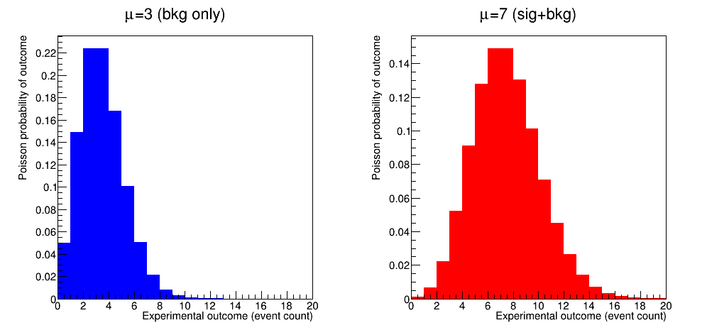
For a given hypothetical physics measurement in which, on average, 3 background events and 4 signal events are expected, Figure shows the Poisson probability distributions for the background-only hypothesis (\(\mu=3\)) and the signal-plus-background hypothesis (\(\mu=7\)). Note that the probabilities assigned by each Poisson model are strictly speaking conditional on the assumed hypothesis: suppose we observe 7 counts in our experiment, then the probability for that outcome depends on the assumed hypothesis (background-only, or signal-plus-background).
The probability of the observed data under a given hypothesis, \(P({\rm data}|H)\) as shown above, is called the Likelihood and conventionally denoted with the symbol \(\mathcal{L}\). The observation \(N=7\) is thus more likely under the \(S+B\) hypothesis than under the \(B\) hypothesis. But is this what we want to know? Or would we rather know \(P(H_{i}|N=7)\), the probability of each hypothesis given the observation of 7 counts? It turns out we don’t have enough information to calculate \(P(H_{i}|N=7)\) from \(L(N=7|H_{i})\). The relation between probabilities with inverted conditionalities is given by Bayes theorem
Thus we need to know the probabilities \(P(H)\) and \(P({\rm data})\) to be able to calculate \(P(H_{i}|N=7)\) from \(L(N=7|H_{i})\). Here, \(P({\rm data})\) is the probability of the data under any hypothesis. If only two hypotheses are considered, as is done here, then \(P({\rm data})\) can be expressed as
applying to law of total probability. Inserting Eq.tprob in Eq.bayes1 gives
where \(i\) can be \(B\) or \(S+B\). To be able to answer the question on what the value of \(P(H_{i}|N=7)\) is, the question of what the probabilities \(P(H_i)\) are then remains: these are the probabilities assigned to either hypothesis prior to the experiment. These prior probabilities can be based on earlier measurements, or can generically be considered to be a prior belief in the theory. Suppose our prior belief in \(H_{S+B}\) and \(H_{B}\) is equal, i.e. \(P(H_{S+B})=P(H_{B})=0.5\), we can then calculate
Thus the observation \(N=7\) strengthens the belief in the \(H_{S+B}\) hypothesis from 0.50 to 0.87, at the expense of the belief in the \(H_{B}\) hypothesis, which is reduced to 0.13.
The interpretation of probabilities
In the discussion so far probabilities assigned to experimental outcomes and to theories have both been used, even though they are conceptually different. Probabilities of observed data can always be interpreted as the fraction of outcome in repeated future experiment, i.e. \(P(N=7|H_{S+B})=0.14\) is interpreted as “in 14% of all future repeated identical experiments we expect the outcome \(N=7\). This frequency-based interpretation of probability is the basis of the classical, or frequentist school of statistics. In the frequentist framework no probabilities can be assigned to theories as there is no concept of repetition for hypotheses. The Bayesian school of statistics on the other hand defines probabilities as a degree of belief, that can also be assigned to hypotheses. As the Bayesian definition of probability no rule-based definition as the frequentist notion does, the probabilities are inherently subjective, although there is large effort in the statistical community to define rule-based prior probabilities that aim to reduce subjective aspects of Bayesian inference.
The different notions of probability are reflected in the type of statements that are made in statistical inference. In the frequentist framework constants of natures are fixed (the Higgs boson either exists or it doesn’t), and no probabilities can be assigned to these. Frequentist statements are thus restricted to probabilities on data. In the Bayesian framework probabilities are assigned to constants of nature (the top quark mass has a 68% probability to be in the interval \(172.2 \pm 0.7\) GeV). As the ultimate goal of any experiment is to make statements on a theory, the choice of the Bayesian of Frequentist framework is largely on the decision at what level to communicate the (numeric) experimental results that form the basis of decision. In the frequentist paradigm probabilities of data are communicated with an objective definition, that can be used for further (subjective) decision making in a later stafe. In the Bayesian paradigm, prior probabilities are inevitable included in the communicated numeric result, and thus communicate a message that contains more (subjective) information than the pure result of the experiment, and give more guidance on the conclusions that should be drawn from the data.
In this context it is intructive to compare the formulation of evidence for discovery of a new particle in both frameworks. In the Bayesian framework evidence for a hypothesis is case as an odds ratio. The ratio of probabilities prior to the experiment defines the prior odds ratio
The posterior odds ratio is defined as the ratio of posterior probabilities, calculated using Eq ref bayes1, where the denominators cancel in the ratio,
The posterior odds ratio can be factorized as the prior odds ratio multiplied with the so-called Bayes factor that contains the experimental information, as shown above. For example, for equal prior odds and an observation \(L({\rm data}|H_{B})=10^{-7}\) and \(L({\rm data}|H_{S+B})=0.5\) the posterior odds ratio becomes 2.000.000:1 in favor of the S+B hypothesis.
In the frequentist paradigm we restrict ourselves to a statement the probability of the observed data, \(L({\rm data}|H_{B})=10^{-7}\) and \(L({\rm data}|H_{S+B})=0.5\) and no notion of prior probabilities on the hypotheses exists, and it is these numbers that constitute final numeric statement. Traditionally, the conclusion that hypothesis B is ruled out is based on the observation of a very small value of \(P({\rm data}|H_{B})\) and a not-so-small value of \(P({\rm data}|H_{S+B})\), and that therefore the signal in the S+B hypothesis is considered ‘discovered’. No formal rules exist to define a discovery threshold, but probality of less than \(2.87 \cdot 10^{-7}\), corresponding to the probability of a \(\ge 5 \sigma\) fluctuation of a unit Gaussian, is traditional considered the threshold for discovery.
In the discussion of discovery threshold one should keep in mind that the probabilistic statement is often only one of the ingredients in the declaration of a discovery: For example for the Higgs boson discovery a \(5 \sigma\) observation was accepted as sufficient evidence, given that the underlying theory was well accepted, whereas much stronger statistical evidence for superluminuous neutrinos was rejected (in retrospect rightfully so), on the basis that they underlying theory was highly implausible, and that a mistake in the experimental analysis was more plausible.
The choice for a Bayesian or Frequentist interpretation of probabilities has a history of long-running discussion in particle physics. Nowadays most particle physics results are reported in the frequentist paradigm, whereas most other science displines use the Bayesian framework. The bulk of this lecture will focus on the construction of likelihood models, which form the basis of both methods. In the discussion of statistical inference methods frequentist methods are discussed in most detail, with the motivation that these are most relevent for todays particle physics students, while highlighting salient differences with Bayesian techniques when applicable.
| [1] | which of course will depend on details of the event selection criteria |
simple hypotheses for distributions
“p-values”
Most particle physics analyses are not simple counting experiments, but study one or more observable distributions that allow to discriminate signal and background.
Probability models for distributions
To deal with distribution in statistic inferences, we must first construct a probability model for distributions. In some cases, the distributions for observable quantities can be derived from the physics theory from first principles, resulting in analytically formulated distributions. In most cases in todays experiments, and in particular at the LHC, predicted distributions for observable quantities are derived from a chain of physics and detector simulations. The output of such simulations is histogram of simulated in events in the observable quantity. An example of such an MC simulation prodiction for a fictious signal and background process is shown in Figures binnedPdf.
While the histograms with simulated signal and background events effectively describe a distribution, the statistical model for such a binned distribution is effectively a series of counting experiments that can be described with a Poisson distribution for each bin
where \(\tilde{b}_i\) and \(\tilde{s}_i\) are the predicted event counts for the background and signal process in bin \(i\) respectively.
Statistical inferences with probability models for distributions
How does the fact that observation is a distribution change statistical inference? In the Bayesian paradigm, the likelihoods of Eq ref La, ref Lb can simply be plugged into Eq ref bayes2, and all further statistical inference procedures are unchanged. The frequentist calculation of \(L(\vec{N}|H_{B})\) also remains unchanged, but raises the question if the probability of the observed data is still relevant when drawing conclusions on the hypotheses considered: \(L(\vec{N}|H_{B})\) is the probability to observe the precise (binned) distribution of data that was recorded. That is usually not what we are interested in. We are interested in the probability to observe this, or any ‘similar’ dataset, e.g. with a few statistical fluctuations w.r.t to the observed data that correspond to the same signal event count, or larger. To introduce a precise, unambiguous notion, of what ‘more signal’ (or more generically ‘more extreme’ in any sense) means in the context of statistical inference, a test statistic is introduced in frequentist inference.
Ordering results by extremity, test statistics and p-values
A test statistic is, generically speaking, any function \(T(x)\) of the observable data \(x\). The goal of a test statistic is that it orders all possible observations \(x\) by extremity: \(T(x)>T(x')\) means that the observation \(x\) is more extreme than observation \(x'\). For example, for a Poisson counting experiment, the trivial choice \(T(x)=x\) defines a useful test statistic that orders all possible observation by extremity as more observed events means more signal for a counting experiment. With the notion of ordering possible outcomes by extremity, comes the concept of \(p\)-values. A \(p\)-value is the probability to obtain the observed data, or more extreme, in future repeated experiments. For example, for the probability to observe 7 counts or more for a Poisson counting experiment with the background hypothesis of the previous example (\(\mu=3\)) is
A \(p\)-value is always specific to the hypothesis under which it is evaluated. When no specification is given, it usually refers the to null-hypothesis, which is for discovery-style analyses the background-only hypothesis.
When the observed data is a distribution, rather than event count, the choice of \(T(x)=x\) will no longer work. We need a test statisticl to quantity if one (multi-dimensional) histogram of observed data \(\vec{N}\) is more extreme than another one. A useful test statistic for distribution is the likelihood ratio test statistic
One can intuitively see that \(\lambda(\vec{N})\) orders datasets according to signal extremity: For a dataset \(N_S\) that is very signal-like \(L(\vec{N_S}|H_{S+B})\) will be large, since the data is probable under this hypothesis, and \(\vec{N_S}|H_{B})\) will be small, since the data is improbable under this hypothesis, hence the ratio will be large. Conversely for a dataset \(N_B\) that is very background-like \(L(\vec{N_B}|H_{S+B})\) will be small, since the data is probable under this hypothesis, and \(L({\vec{N_B}}|H_{B})\) will be large, since the data is improbable under this hypothesis, hence the ratio will be large.
With a likelihood-ratio test statistic, frequentist \(p\)-values can be calculated for observable data distributions or arbitrary complexity as the test statistic \(T(\vec{x})\) maps any dataset \(x\) into a single number \(T(x)\), reducing the \(p\)-value calculation to an integral over the expected test statistic distribution under a given hypothesis
where \(f(T|H_{i})\) is the expected distribution of values of the test statistic \(T\) under the hypothesis \(H_i\). Note that the Poisson example of Eq ref poisT follows from the general form of Eq ref Tdist with the choice \(T(N)=N\) and \(H_i = {\rm Poisson}(\mu=3)\), where integration was replaced with a summation because of the integer nature \(T(N)=N\). Figure ref tsdist illustrates the concept of the distribution of the test statistic and its relation to the definition of the p-value.
![]()
A practical complication in the calculation of \(p\)-values for distribution is that, unlike the Poisson example with \(T(x)=x\) where distribution of \(T(x)\) is known because it simply the Poisson distribution of \(x\) itself, the distribution \(f(T|H_i)\) is generally not known. A simple, but but computionally expensive solution is the estimate the distribution \(f(T|H_i)\) from toy Monte Carlo simulation: a histogram of the \(T(x)\) values from ensemble of toy datasets \(x\) drawn from the hypothesis \(H_i\) will approximate the distribution \(f(T|H_i)\). For certain choices of \(T(x)\) analytical distributions are known under asymptotic conditions, and will be discussed in Section ref composite
While not discussed further in these lecture notes, for situations where analytical prescriptions are known for the distribution of observable quantities \(x\), the concept of a probability model can be extended into the concept of a probability density model \(f(x)\) where \(\int f(x) dx \equiv 1\) and the definite integral \(\int_a^b f(x) dx\) represents the probability to observe an event in the observable range \(a<x<b\). All of the statistical inference techniques discussion in this section can be identically executed using such probability density function instead of probability models.
Hypothesis tests as basis for event selection
“Optimal event selection and machine learning”
In the example Poisson model studied so far, we have focused on the statistical analysis of a counting experiment that is performed in an otherwise unspecified event selection. Designing an optimal event selection for a particular signal problem is nevertheless a core element of particle physics data analysis, and usually precedes statistical analysis of the selected event. The reason it is discussed in this lecture after an introduction on test statistics is that the theoretical basis for optimal event selection is closely connected to the likelihood ratio test statistic. In fact, with the introduction of the likelihood ratio test statistic we have already solved optimal the event selection problem for simply hypotheses: any selection defined by a lower cut on the likelihood ratio test statistic
will select on the most signal-like events in the total collection, only leaving the issue of deciding on cut the value that will define the desired purity of the selection.
The general concept of event selection relates to the statistical subject of classical hypothesis testing. In classical hypothesis testing we define two competing hypothesis, traditional called the null hypothesis \(H_0\), representing the background hypothesis in event selection, and the alternate hypothesis \(H_1\) representing the signal hypothesis in event selection. The goal of an event selection is to select as many signal events as possible, while rejecting as many background events as possible. The succes at meeting these competing goals is quantified in two measures:
- The ‘type-I’ error rate \(\alpha\), also called the size of the test. This rate represent the false positive rate, e.g. unjustly convicted suspects in trial, or background events mistakenly accepted in the signal selection.
- The ‘type-II’ error rate \(\beta\), where \(1-\beta\) is also called the power of the test. This rate represent the false negative rate, e.g mistakenly acquitted criminals or signal events mistakenly not selected in the signal region.
In general classical hypothesis testing, these goals are treated asymmetrically to construct an unambiguous optimization goal: the false positive rate \(\alpha\) is usually fixed to user-defined acceptable level (e.g. 5%), and the false negative rate \(\beta\) is then minimized. In HEP event selection problems on the other hand, no fixed value for \(\alpha\) is typically assumed, instead the optimal tradeoff between \(\alpha\) and \(\beta\) is chosen with the aid of a figure of merit that quantifies the performance of the statistical analysis of events in the signal region, such as the expected significance of the signal.
In 1932 Neyman and Pearson demonstrated that the optimal event selection for a problem with two competing hypotheses ( \(H_0\) = background and \(H_1\) = signal) the region \(W\) that minimizes the type-II error rate \(\beta\) for a given type-I error rate \(\alpha\) is defined by a contour of the likelihood ratio,
which is form very similar to the likelihood ratio test statistic \(\lambda(\vec{x})\) of Eq. ref lambda. The NP lemma also proves that \(\lambda(\vec{x})\) is an optimal test statistic, i.e. no information that distinguishes \(H_{S+B}\) from \(H_{B}\) is lost in the compactification \(\vec{x} \to T(\vec{x})\).
Even though Eq. ref NPlemma provides the optimal event selection for a signal and background events characterized by hypotheses \(H_1\) and \(H_0\), it is not always a practical criteria: it requires that the probabilities \(L(x|H_1)\) and \(L(x|H_0)\) are calculable for any \(x\). In practice the only information available on \(H_0\) and \(H_1\) is an ensemble of simulated events \(x\) drawn from each hypothesis. Except for low dimensions of \(x\), where a histogram in \(x\) can be populated for the full phase space, the ensembles of simulated events do not allow to calculate the probabilities \(L(x|H_1)\) and \(L(x|H_0)\) that are required to use Eq. NPlemma.
Instead a different strategy can be followed that is aimed at approximating the optimal decision boundary with an Ansatz function with parameters that can be “machine learned”, or otherwise inferred from training data.
Composite hypotheses (with parameters) for distributions
“Confidence intervals and maximum likelihood”
All statistical techniques discussed so far were based on simple hypotheses in which the distribution of observables is fully specified. In other words, simple hypotheses cover situations in which there are no known uncertainties in the model that is intended to describe the data. Most practical problems in physics analysis however involve a multitude of uncertain effects, ranging from uncertain calibration constants to unknown signal cross-sections. These uncertainties are accounted for in the concept of composite hypotheses, which can have one or more parameters whose value is a priori not precisely known. To illustrate the concept of composite hypothesis we extend the Poisson counting experiment of the previous section into a composite hypothesis by introducing the signal rate as a model parameter, rather than having it as a known constant [2]
Figure ref poisson_composite shows the probability distribution for possible counting outcomes of Eq. ref poisson_sb for various assumed values of its parameter \(s\). A composite hypothesis can have any number or type of parameters. Parameters are usually distinguished in two types: “parameters of interest”, and “nuisance parameters”. A parameter of interest (POIs) is any parameter that one is ultimately interested in, e.g. the reported physics quantity of the analysis. Many analyses have a single parameter of interest, but multiple POIs can also occur, for example in a measurement of Higgs boson couplings each coupling will have its own POI. Nuisance parameters are then implicitly defined as all other model parameters that are not of interest. Typically nuisance parameter described uncertainties in detector modelling (calibration uncertainties, efficiencies) and theoretical modelling (factorization/normalization scales). We will now first consider composite hypothesis with a single parameter of interest and no nuisance parameters, returning to the issues of nuisance parameters in Section ref np. Where statements on simple hypotheses were limited to \(P(data|H)\) and \(P(H|data)\) composite hypothesis offer a new range of probabilistic statements that can be made on the model parameter (of interest):
- Parameter value and variance estimation: e.g. \(s = 4.3 \pm 0.7\)
- Confidence intervals: e.g. \(s < 7.7\) at 95% C.L.
- Bayesian credible intervals: e.g \(s < 7.6\) at 95% credibility
Parameter estimations determines for which value \(\hat{s}\) of the parameter \(s\) the observed data is most probable. A parameter variance estimate determines the variance of such a point estimate, where the variance is defined in the usual way as \(\left<s^2\right> - \left<s\right>^2\). The variance expresses how much the point estimate \(\hat{s}\) will vary in repeated identical experiments. Confidence intervals and Bayesian credible intervals convey conceptually similar information, but with different definitions and properties.
Maximum Likelihood parameter estimation
The procedure to obtain the value \(\hat{s}\) of a model parameter \(s\) for which the data is most probably is called the method of maximum likelihood. The procedure entails finding the value \(s\) for which \(L(s)\) is maximal. For a simple likelihood like that of Eq. ref poisson_sb the estimation \(s\) can be performed analytically by differentiation, for more complex likelihood expressions the estimations is performed numerically, where it is customary to find the maximum of \(-\log L(s)\) rather than the maximum of \(L(s)\) as it is numerically more stable:
The standard notation is that \(\hat{p}\) is the (maximum likelihood) estimator of parameter \(p\): it represents value of \(p\) that is obtained by running the (maximum likelihood) estimation procedure on that parameter. Figure ref poisson_shat shows the value of the negative log-likelihood \(-\log L(N=7|s)\) for the Poisson model of Eq. ref poisson_sb where \(\hat{b}=5\). Note that the \(L(N|s)\) is continuous in \(s\), even though \(N\) only takes integer values. The maximum likelihood \(\hat{s}\) is the value of \(s\) for which \(-\log L(s)\) is minimal, i.e. \(\hat{s}=2\).
Maximum likelihood estimators are commonly used because they have desirable properties: ML estimators are in general
- Consistent: you get the correct answer in the limit of infinite statistics
- Mostly unbiased: the bias is proportional to \(1/N\), which becomes small compared to the estimated uncertainty proportional to \(1/\sqrt{N}\) for moderate \(N\).
- Efficient for large :math:`N`: The actual variance of ML estimator \(s\) will not be larger than \(\left<s^2\right> - \left<s\right>^2\).
- Invariant: A transformation of parameters will not changes the answer, i.e. \((\hat{p})^2 = \widehat{p^{2}}\).
In particular, the Maximum Likelihood Efficiency theorem states that a ML estimator will be efficient and unbiased for a given composite hypothesis if an unbiased efficient estimator exists for that hypothesis (proof not discussed here).
Parameter variance and the central limit theorem
It is important to note that term “uncertainty on a parameter estimate” is not uniquely defined. Multiple procedures exist that define intervals on parameters, that may yield different results depending on the underlying distributions. One of the common procedure to define an uncertainty is to take the square-root of the variance of the parameter, defined as
For Gaussian distributions an \(1 \sigma\) interval defined by \(\sqrt{V}\) will contain 68% of the distribution. For other distributions this fraction may be different, nevertheless the variance is a well-defined distribution for almost any distribution [3]. In practice most distributions that do not suffer from very low statistics are approximately Gaussian due to the Central Limit Theorem CLT) which states that the sum of \(N\) independent measurement \(x_i\), each taken from a distribution of mean \(m_i\) and a variance \(V_i\) has an expectation value \(\left< x \right> = \sum_i \mu_i\), a variance \(V_x = \sum_i V_i\) and becomes Gaussian in the limit of large \(N\). Figure ref clt demonstrates this property of the CLT for a sum of 2,3,12 measurements \(x_i\) , each drawn from a very non-Gaussian flat distribution, where the \(N=12\) case already results in a very Gaussian distribution. The variance \(V_p\) of a parameter estimate \(\hat{p}\) can be obtained with the Maximum Likelihood Variance estimator
The ML variance estimator is only efficient, i.e it will not estimate variance larger than the true variance, when the ML estimator of \(p\) is unbiased, which is usually the case at moderate to high statistics.
Confidence intervals
Another approach to defining intervals on parameters is the frequentist confidence intervals. The advantage of such fundamental methods is that they make no assumptions on the distribution (and are therefore useable in very low statistics cases) and return calibrated probabilistic statements, i.e. a 68% confidence interval definition does not rely on the fact that the underlying distribution is Gaussian.
The classical, or frequentist confidence intervals arrives at this calibrated and distribution-independent statement as follows. Given a probability model \(f(x|\mu)\) with a single parameter \(\mu\), the expected distribution of the observable \(x\) is mapped out for all values of \(\mu\) (see Fig ref nmconstr a). Next, an acceptance interval is defined for the distribution of \(x\). A simple and common way to define an acceptance interval is to take a 68% central interval, i.e. defined the interval such that 16% of the distribution sits on both the left and right side of the defined interval (Fig ref nmconstr b). Then these accepted regions in \(f(x|\mu)\) are connected for all values \(\mu\) ((Fig ref nmconstr c). This region in \(f(x|\mu)\)-vs-mu space is called the confidence belt. To defined a confidence interval on \(\mu\), a line at the observed value \(x_{obs}\) is intersected with the confidence belt to obtain the interval \([\theta_{-},\theta_{+}]\). The result of this procedure, called the Neyman Construction, is that the true value of \(\theta\), guaranteed to be contained in 68% of repeated measurements of this type, without assumptions on the distribution \(f(x|\mu)\). Confidence intervals can also take different shapes. For example, when instead of a 68% central interval, a 95% lower interval is chosen as acceptance region in \(f(x|\mu)\), the resulting confidence interval on \(\theta\) will be a 95% upper limit. Confidence intervals thus provide great flexibility in the form in which results can be formulated, dependening on the ordering rule, the procedure that is chosen to define an acceptance interval on \(f(x|\mu)\).
Note that frequentist confidence intervals strictly make no probabilistic statement about the true value of \(\mu\). In the frequentist concept of probabilities the true value of \(\mu\) is fixed, but unknown, and no probability distribution can be assigned to it. Instead the interval estimation procedure is constructed such that the intervals it produces are guaranteed to contain in exactly 68% (or 95%) of the repeated identical measurements the true (but unknown) value.
Confidence intervals using likelihood ratios
The text-book case of the construction of confidence intervals as shown in Fig ref nmconstr works only for simple probability models with a single observable \(x\). To define confidence intervals on probabity models where the observable \(x\) is not a single number, but a (multi-dimensional) distribution, the likelihood ratio technique introduced earlier in Section 3.3 comes to the rescue. Instead of taking an ordering rule that defines an interval in \(f(x|\mu)\), a new ordering rule is introduced that instead defines an interval on a likelihood ratio based on \(f(x|\mu)\)
to define a confidence belt. Whereas the text-book confidence belt of Fig ref nmconstr provided an intuitive graphical illustration of the concept of acceptance intervals on \(x\) and confidence intervals in \(\mu\), a confidence belt based on a likelihood-ratio ordering rule may seem at first more obscure, but in reality isn’t. Figure ref nmconstr2 compares side-by-side the text-book confidence belt of \(f(x|\mu)\) with a LLR-based confidence belt of \(\lambda(\vec{N}|\mu)\). We observe the following differences
- The variable on the horizontal axis is \(\lambda(\vec{N}|\mu)\) instead of \(f(x|\mu)\). As \(\lambda(\vec{N}|\mu)\) is a scalar quantity regardless of the complexity of the observable \(\vec{N}\) this allows us to make this confidence belt construction for any model \(f(\vec{N}|\mu)\) of arbitrary complexity.
- The confidence belt has a different shape. Whereas the expected distribution \(f(x|\mu)\) is typically different for each value of \(\mu\), the expected distribution of \(\lambda(\vec{N}|\mu)\) typically is independent of \(\mu\). The reason for this is the asymptotic distribution of \(\lambda(\vec{N}|\mu)\) that will be discussed further in a moment. The result is though that a LLR-based confidence belt is usually a rectangular region starting at \(\lambda=0\).
- The observed quantity \(\lambda(\vec{N}|\mu)_{obs}\) depends on \(\mu\) unlike the observed quantity \(x_{obs}\) in the textbook case. The reason for this is simply the form of Eq.ref{eq:llr} that is an explicit function of \(\mu\). Asymptotically the dependence of \(\lambda(\vec{N}|\mu)\) on \(\mu\) is quadratic, as shown in the illustration.
The confidence belt construction shown in Fig ref nmconstr2, when rotated 90 degrees counterclockwise looks of course very much like an interval defined by a rise in the likelihood (ratio), as is done by MINUITS MINOS procedure, and that correspondence is exact in the limit of large statistics. This last observation brings about an important point: in the limit of large statistics, the ‘simple’ procedure of defining an interval by a rise in the likelihood ratio defines a proper frequentist confidence interval with its desirable properties: the result is independent of the distribution and the quoted (68 or 95%) confidence level is calibrated. This asymptotic correspondence of the completely general (and potentially) expensive Neyman Construction procedure with its desirable calibration properties and asymptotic and computationally light likelihood ratio interval procedure occurs when Wilks theorem is satisfied, i.e that the distribution of \(\lambda(\vec{N}|\mu)\) for data sampled under the hypothesis \(\mu\) is asymptotically distributed as a \(\chi^2\) distribution, and therefore is independent of \(\mu\). Note that this condition does not imply that the likelihood ratio as function of \(\mu\) is exactly parabolic, thus the interpretation of asymmetric MINOS error as frequentist confidence intervals is correct as long as Wilks theorem is met. When in doubt, one can check this requirement by verifying that the distribution of \(\lambda(\vec{N}|\mu)\) values from a suitable large sample of toy datasets follows the asymptotic \(\chi^2\) distribution, as is shown in Figure ref wilks.
Confidence intervals with boundaries
As frequentist confidence intervals make statements on the frequency of measured values and do not aim to interpret these measurement values as a probabilistic statement on constants of nature as a Bayesian procedure does, the occurence of intervals that (partially) cover unphysical values do not pose a problem. A classical situation of this type is the Poisson counting experiment where the observed event count is less than the expected background event count. For example, for a counting experiment with 10 expected background events and 3 expected signal events, an observation of 8 events is entirely unproblematic, although the resulting parameter estimate of -2 signal events is sometimes frowned upon. The key to interpreting such a result is to realize that -2 signal events is strictly the outcome of a measurement procedure, and is expected to occur at some frequency. If the negative fluctuation is substantial, e.g. 5 observed for 10 expected background, it can happen that the resulting interval estimate only brackets negative values for the signal count, in other words, all signal counts greater than 0 are excluded, at 95% confidence level. Also this is, strictly speaking, not a problem, as the true value is outside the quoted interval in 5% of the measurements by construction. Nevertheless, many physicists are uncomfortable quoting a result of this type as the final outcome as the result of a physics measurement.
It is possible to adjust the construction procedures of confidence intervals such that such unphysics intervals cannot occur and yet respect the essential calibration property of the Neyman construction - namely that the reported intervals are guaranteed to contain the true value in 68% or 95% of the cases. The key to accomplish this is to only modify the ordering rule, but leave the Neyman construction itself (which guarantees the calibration) unchanged. To do so the standard likelihood ratio ordering rule, encoded by
is replaced by
The ordering rule \(\tilde{t}\) changes the interpretation of observations with \(\hat{\mu}<0\). Consider the ordering rule for the no-signal hypothesis (mu=0) for an observation of \(\hat{\mu}=-2\): The traditional test statistic \(t_{\mu}\) will consider this observation to be inconsistent with the no-signal hypothesis: \(\log(L(x|0)/L(x|-2))\) will be larger than zero. At as sufficiently negative \(\hat{\mu}\), when \(t_{\mu}\) becomes larger than 0.5 for \(\mu=0\), the points \(\mu\ge 0\) will be excluded from a 68% confidence interval and once it becomes larger than 2, the points \(\mu\ge 0\) will also be excluded at 95% C.L.
The modified test statistic \(\tilde{t}_{\mu}\) will on the other hand consider any observation with \(\hat{\mu}<0\) to be maximally consistent with the no-signal hypothesis: \(\log(L(x|0)/L(x|0))\) will be exactly zero for any observation with \(\hat{\mu}<0\)! The effect of this modification on the resulting confidence belt is that \(\mu=0\) is inside the confidence interval corresponding to any observation with \(\hat{\mu}<0\) , hence no downward fluctuations w.r.t the background estimate will result in the exclusion of \(\mu=0\). In practice, small positive values of \(\mu\) will also not be excluded, hence any observation with \(\hat{\mu}<0)\) will result in a confidence interval \([0,\mu_{+}]\), with the size of the confidence interval decreasing with decreasing \(\hat{\mu}<0)\).
Observations of event counts much larger than the background estimate, on the other hand, do not trigger such special handling. Thus the observation of a very large positive event count will exclude \(\mu=0\) from the confidence interval, and result as usual in a two-side confidence interval \([\mu_{-},\mu_{+}]\), corresponding to a measurement-style result. The point where the transition from a one-sided interval of the from \([0,\mu_{+}]\) transitions into a two-sided interval \([\mu_{-},\mu_{+}]\) is automatically determined by the procedure. In the HEP literature the confidence intervals constructed with an ordering rule based on the modified likelihood ratio \(\tilde{t}_{\mu}\) is usually called the ‘modified frequentist procedure’, or Feldman-Cousins, and is considered to be a ‘unified’ procedure as the transition from upper limits to two-sided intervals is automatically determined. As for \(t_{\mu}\), asymptotic distributions for the modified test statistic \(\tilde{t}_{\mu}\) are known, and are discussed in detail in [X].
| [2] | To facilitate the distinction between symbolic constant expressions (a known background) and symbolic parameters (an unknown background) all constant symbols are marked with a tilde: i.e. \(\tilde{a}\) is constant expression, whereas \(a\) is a parameter. |
| [3] | An notable example of a distribution that has no well-defined mean or variance is the non-relativistic Breit-Wigner distribution. |
Bayesian credible intervals
The introduction of composite hypotheses in Bayesian statistics transforms Bayes theorem from an equation calculating probabilities for hypothesis, into an equation calculating probability densities for model parameters, i.e.
Statistical inference with nuisance parameters
“Fitting the background”
In all examples of this course so far, we have only considered ideal experiments, i.e. experiments that have associated systematic uncertainties originating from experimental aspects or theoretical calculations. This section will explore how to modify statistical procedures to account for the presence of parameter associated to systematic uncertainties, whose values are not perfectly known.
What are systematic uncertainties
The label systematic uncertainty strictly originates in the domain of the (physics) problem that we are trying to solve, it is not a concept in statistical modelling. In practice, a systematic uncertainty arises when there effect whose precise shape and magnitude is not know affects our measurement, hence we need to have some estimate of it. A common approach is that we aim capture the unknown effect in one or more model parameters, whose values we then consider the not perfectly known. A good example is a detector calibration uncertainty that affects an invariant mass measurement. If the assumed calibration in the statistical analysis is different from the true (but known) calibration of the detector the measurement will be off my some amount. In most cases some information is available on the unknown calibration constant, in the form of a calibration measurement with an associated uncertainty “the energy scale of reconstructed jets has a 5% uncertainty”. An example of a systematic uncertainty arising from theory is a cross-section uncertainty on a background process in a counting experiment. In both these cases the goal is propagate the effect of the uncertainty on the parameter associated with the theoretical uncertainty to the measurement of the parameter of interest. In the discussion of systematic uncertainties there are hence two distinct aspects that should be distinguished
- Identifying which are the degrees of freedom associated with the conceptual systematic uncertainty, and implement these as model parameters
- Account for the presence of these uncertain model parameters in the statistical inference.
The first aspect is a complex subject that is strongly entangled in the physics of the problem that one aims to solve and is discussed in detail in the next section, whereas the second subject is purely on statistical procedure, and is discussed in this section following a simple example likelihood featuring one or more such “nuisance parameters”.
Treatment of nuisance parameters in parameter point and variance estimation
To illustrate the concept of nuisance parameter treatment in point and variance estimation, we can construct a simple extension of the Poisson counting example introduced in Equation X33, by now considering the background that was previously assumed to exactly known, to be unknown, and measurement from a second counting experiment that only measures the backgroundfootnote{The experiment is constructed such that the background rate measurement in the control regions is three times the expected background rate in the signal region.}
The likelihood function of Eq. ref PoissonSB can be used to construct a 2-dimensional measurement of both \(s\) and \(b\) following the procedures outline in Section X, but given that we are now only interested in the signal rate \(s\) and not in the background rate \(b\), the goal is to formulate a statement on \(s\) only, while taking into account the uncertainty on \(b\). Figure ref PoissonSB2D shows the 2-dimensional likelihood function for \(L(s,b)\) for an observation of \(N_{SR}=10, N_{CR}=10\). A likelihood \(L(s)\) without nuisance parameters that assumes \(b=5\) corresponds to the slice of the plot indicated at the dashed line and will estimate \(\hat{s}=5\), where the maximum likelihood is found in that slice. A likelihood \(L(s,b)\) with \(b\) as a nuisance parameter will instead find the minimum \(\hat{b}=3.3,\hat{s}=6.7\), with the effect of the nuisance parameter ostensibly taken into account.
The effect of the nuisance parameter \(b\) on the variance estimate of \(s\) comes in through the extension of the one-dimensional variance estimator into a multidimensional covariance estimator
If the estimators of \(s\) and \(b\) are correlated, the off-diagonal elements of the matrix in Eq. ref covariance are non-zero and the variance estimates on \(s\) using \(V(s)\) and \(V(s,b)\) will differ. This difference in variance is visualized in Fig ref covsb that shows a contour of \(L(s,b)\) in the \(s,b\) plane assuming a Gaussian distribution for a scenario where the estimates of \(s,b\) are somewhat anti-correlated (left) and uncorrelated (right). The square-root of the variance estimate on \(s\) using \(V(s)\) corresponds to the distance between the intersection of the the line \(b=\hat{b}\) with the likelihood contour (red line). The square-root of the variance estimate on \(s\) using \(V(s,b)\) corresponds the size of the box that encloses the the contour. If the estimators of \(s\) and \(b\) are uncorrelated, both methods will return the same variance, reflecting that the uncertainty on \(b\) has no impact on the measurement of \(s\). If on the other had the estimators of \(s\) and \(b\) are correlated, the variance estimate from \(V(s,b)\) will always be larger than the estimate from \(V(s)\), reflecting the impact of the uncertainty on \(b\) on the measurement on \(s\).
Treatment of nuisance parameters in hypothesis testing and confidence intervals
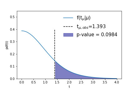
The calculation of \(p\)-values for hypothesis testing in models with a parameter of interest \(\mu\), but without nuisance parameters is based on the distribution of the test statistic \(p_{\mu} = \int_{t_{\mu,obs}}^{\infty} f(t_{\mu}|\mu) dt_{\mu}\) where \(t_\mu\) is the test statistic (usually a likelihood ratio), \(f(t_\mu|\mu)\) is the expected distribution of that test statistic and \(t_{\mu,obs}\) is the observed value of the test statistic. With the introduction of a generic nuisance parameter \(\theta\), i.e. \(L(\mu) \to L(\mu,\theta)\) the distribution of a test statistic based on that likelihood (ratio) will generallly also depend on \(\theta\)
and hence the question now is, what value of \(\theta\) to assume in the distribution of \(t_{\mu}\)? Fundamentally, we want to reject the hypothesis \(\mu\) at \(\alpha\%\) C.L. only if \(p_{\mu}<1-\alpha\) for any value of :math:`theta`. In other words, if there is any value of \(\theta\) for which the data is compatible with hypothesis \(\mu\) we do not want to reject the hypothesis. This approach appears a priori extremely challenging both technically (performing the calculation for each possible value of \(\theta\)) also conceptually (one should really consider values of \(\theta\) that are itself excluded by other measurements), but it turns out that with a clever choice of \(t_{\mu}\) the statistical problem becomes quite tractable. The key is to replace the likelihood ratio test statistic with the profile likelihood ratio test statistic
where the symbol \(\hat{\hat{\mu}}\) represents the conditional [4] maximum likelihood estimate of \(\theta\). Note that the profile likelihood ratio test statistic \(\Lambda_{\mu}\) does explicitly not depend on the Likelihood parameter \(\theta\) as both \(\hat{\theta}\) and \(\hat{\hat{\theta}}\) are determined by the data. In the limit of large statistics the distribution of the test statistic \(f(\Lambda_{\mu}|\mu_{true},\theta_{true})\) follows a \(\chi^2\) distribution, just like the distribution of \(t_{\mu}\). This is nice for two reasons: first it allows us to reuse the formalism developed for the construction of confidence intervals based on \(t_{\mu}\) to be recycled for \(\Lambda_{\mu}\) by simply replacing the test statistic. Second it means that \(f(\Lambda_{\mu}|\mu_{true},\theta_{true})\) is asymptotically independent of the true value of both \(\mu_{true}\) and \(\theta_{true}\) so that the interval based on \(\Lambda_{\mu}\) convergence to a proper frequentist interval even in the present of nuisance parameters in the asymptotic limit.
It is instructive to compare the plain likelihood ratio \(t_{\mu}\) and profile likelihood ratio \(\Lambda_{\mu}\) for an example model: the distribution of an observable \(x\) that is described by a Gaussian signal and and order-6 Chebychev polynomial background. The corresponding likelihood function has one parameter of interest, the signal strength, and 6 nuisance parameters, the coefficients of the polynomial. Figure ref plrdemo shows the distribution of the plain likelihood ratio (blue, top) and the profile likelihood ratio (red, bottom). As the likelihood model with floating nuisance parameters is generally more consistent with the observed data for each assumed value of the signal strength (as the polynomial background can be configured to peak or dip in the signal region), the confidence interval of the profile likelihood ratio is wider than that of the plain likelihood ratio, reflecting the additional uncertainty introduced on the measurement of the signal strength by the fact that the background shape is not perfectly known.
| [4] | Where the condition is that the POI is fixed at the value \(\mu\), rather than allowed to float to the value \(\hat{\mu}\) in the minimization, as is the case in the minimization of the unconditional estimate \(\hat{\theta}\) |
Tools for Model Building and Good Practices
This section discusses the specific tools for recommended for building valid and robust statistical models. The RooFit pacakge is core to data modeling in ROOT.
We begin with a discussion of the RooFit philosophy - we want a single language for all measurements: common tools & joint model building (other tools) followed by a description of the RooFit language basics, and the workspace. A series of tools for building & manipulating models built using RooFit as a foundation are described with some links and general usage. Finally a list of good practices are presented regarding issues such as modeling systematics, uncertainties, and model cleaning among others.
RooFit
RooFit - a model building language
The main feature of the design of the RooFit/RooStats suite of statistical analysis tools is that the tools to build statistical models and the tools to perform statistical inference are separate, but interoperable. This interoperability is universally possible because all statistical inference is based on the likelihood function.
The goal is that all tools in the RooStats suite can analyse any model built in RooFit. The interoperability is facilitated in practice by the concept of the workspace (RooFit class RooWorkspace) that allows to persist statistical models of arbitrary complexity into ROOT files and thus allow to separate the model building phase and the statistical inference phase of a data analysis project both in space and time
RooFit basics
This section will cover the essentials of the RooFit modelling language, which wil aid in the understanding of the role of higher level modelling tools and model manipulation.
The key concept of RooFit probability models is that all components that form the mathematical expression of a probability model or probability density function are expressed in separate C++ objects. Base classes exist to represent e.g. variables, functions, normalised probability density functions, integrals of function, datasets, and implementations of many concrete functions and probability density functions are provided.
The examples below show how a Gaussian and Poisson probability model are built by constructing first the component objects (the parameters and observables), and the the probability (density) functions.
// Construct a Gaussian probability density model
RooRealVar x("x","x",0,-10,10) ;
RooRealVar mean("mean","Mean of Gaussian",0,-10,10) ;
RooRealVar width("width","With of Gaussian",3,0.1,10) ;
RooGaussian g("g","Gaussian",x, mean,width) ;
// Construct a Poisson probability model
RooRealVar n("n","Observed event cont",0,0,100) ;
RooRealVar mu("mu","Expected event count",10,0,100) ;
RooPoisson p("p","Poisson",n, mu) ;
|
# Construct a Gaussian probability density model
x = ROOT.RooRealVar("x","x",0,-10,10)
mean = ROOT.RooRealVar("mean","Mean of Gaussian",0,-10,10)
width = ROOT.RooRealVar("width","With of Gaussian",3,0.1,10)
g = ROOT.RooGaussian("g","Gaussian",ROOT.RooArgSet(x), mean,width)
# Construct a Poisson probability model
n = ROOT.RooRealVar("n","Observed event cont",0,0,100)
mu = ROOT.RooRealVar("mu","Expected event count",10,0,100)
p = ROOT.RooPoisson("p","Poisson",n, mu)
|
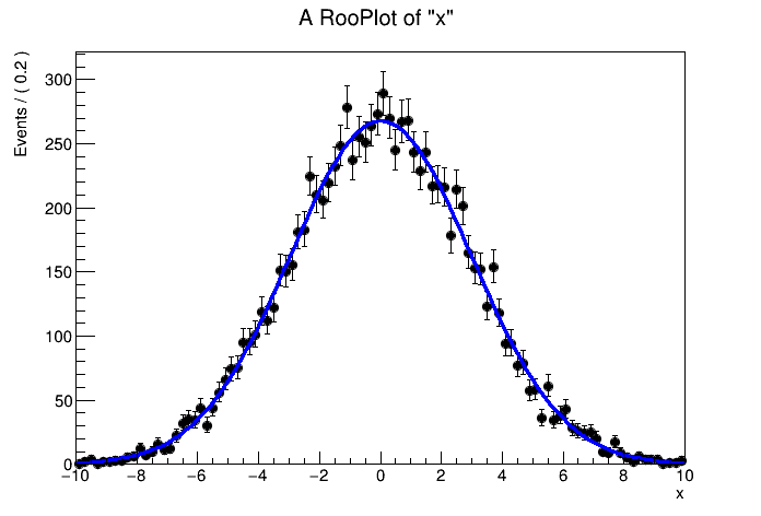
RooFit implements all basic functionality of statistical models: toy data generation, plotting, and fitting (interfacing ROOTs minimisers for the actual -logL minimisation process).
// generate unbnined dataset of 10k events
RooDataSet* toyData = g.generate(x,10000) ;
// Perform unbinned ML fit to toy data
g.fitTo(*toyData) ;
// Plot toy data and pdf in observable x
RooPlot* frame = x.frame() ;
toyData->plotOn(frame) ;
g.plotOn(frame) ;
frame->Draw() ;
|
# generate unbnined dataset of 10k events
toyData = g.generate(ROOT.RooArgSet(x),10000)
# Perform unbinned ML fit to toy data
g.fitTo(toyData)
# Plot toy data and pdf in observable x
frame = x.frame()
toyData.plotOn(frame)
g.plotOn(frame)
frame.Draw()
|
As the likelihood function plays an important role in many statistical techniques, it can also be explicitly constructed as a RooFit function object for more detailed control
// Create Likelihood function L(x|mu,sigma) for all x in toy data
RooAbsReal* nll = g.createNLL(*toyData) ;
// ML estimation of model parameters mean,width
RooMinimizer m(*nll) ;
m.migrad() ; // Minimization
m.hesse() ; // Hessian error analysis
// Result of minimisation and error analysis is propagated
// to variable objects representing model parameters
mean.Print() ;
width.Print() ;
// Visualize likelihood L(mu, sigma)
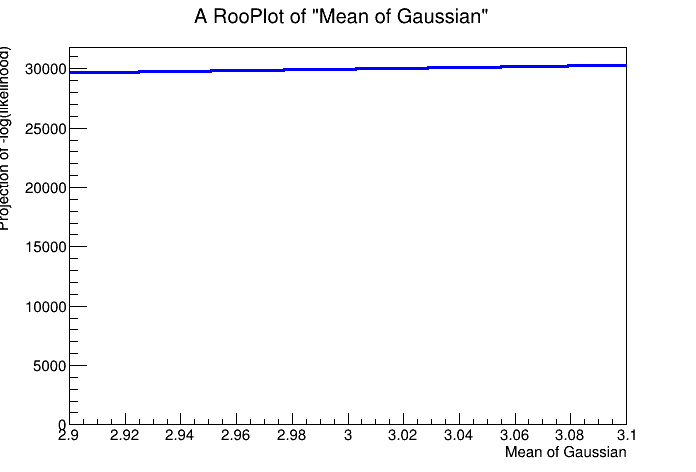
// at sigma = sigma_hat in range 2.9<mu<3.1
RooPlot* frame2 = mean.frame(2.9,3.1) ;
nll->plotOn(frame2) ;
frame2->Draw() ;
|
# Create Likelihood function L(x|mu,sigma) for all x in toy data
nll = g.createNLL(toyData)
# ML estimation of model parameters mean,width
m = ROOT.RooMinimizer(nll)
m.migrad() # Minimization
m.hesse() # Hessian error analysis
# Result of minimisation and error analysis is propagated
# to variable objects representing model parameters
mean.Print()
width.Print()
# Visualize likelihood L(mu, sigma)
# at sigma = sigma_hat in range 2.9<mu<3.1
frame2 = mean.frame(2.9,3.1)
nll.plotOn(frame2)
frame2.Draw()
|
RooFit implements a very wide range of options to tailor models and their use that are not discussed here in the interest of brevity, but are discussed in detail here <insert_link>. RooFit also automatically performs an optimisation of the computation strategy of each likelihood before each use, so that users that build models generally do not need to worry about specific performance considerations when expression the model. Example optimisations include automatic detection of unused dataset variables in a likelihood, automatic detection of expression that only depend on (presently) constant parameters and caching and lazy evaluation of expensive objects such as numerical integrals. The following links provide further information on a number of RooFit related topics
- Guide to the RooFit workspace and factory language <LINK>
- Guide to (automatic) computational optimizations in RooFit <LINK>
- Guide to writing your own RooFit PDF classes <LINK>
RooFit workspace essentials
The key to the RooFit/RooStats approach of separating model building and statistical inference is the ability to persist built models into ROOT files and the ability to revive these with minimal effort in a later ROOT session. This ability is powered by the RooFit workspace class, in which built models can be important, which organises the persistence of these models, regardless of their complexity
// Saving a model to the workspace
RooWorkspace w("w") ;
w.import(g) ;
w.import(p) ;
w.import(*toyData,RooFit::Rename("toyData")) ;
w.Print() ;
w.writeToFile("model.root") ;
// ————————————————
// Reviving a model from a workspace
TFile* f = TFile::Open("model.root") ;
RooWorkspace * w = (RooWorkspace*) f->Get("w") ;
RooAbsPdf* g = w->pdf("g") ;
RooAbsPdf* p = w->pdf("p") ;
RooDataSet* toyDatata = w->data("toyData") ;
|
# Saving a model to the workspace
w = ROOT.RooWorkspace("w")
getattr(w,'import')(g)
getattr(w,'import')(p)
getattr(w,'import')(toyData,ROOT.RooFit.Rename("toyData"))
w.Print()
w.writeToFile("model.root")
# ————————————————
# Reviving a model from a workspace
f = ROOT.TFile.Open("model.root")
w = f.Get("w")
g = w.pdf("g")
p = w.pdf("p")
toyDatata = w.data("toyData")
|
The code example above, while straightforward highlights a couple of important points
- Reviving a model or dataset is always trivial, typically 3-4 lines of code depending on the number of objects that must be retrieved from the workspace, even for large workspaces e.g. full Higgs combinations that can contain over ten thousand component objects.
- Retrieval of objects (functions, datasets) is indexed by their internal object, as giving to them in the first C++ constructor argument (all RooFit object inherit from ROOT class TNamed, which identical behaviour).
- For objects where the model building user did not explicitly specify the objects intrinsic name, like the toyData object in the example above, it is possible to rename the object to a given name after the fact. The most convenient path to do this is to do this upon import in the workspace, as shown in the code example above.
The ModelConfig interface object
Since model and data names do not need to conform to any specific convention, the automatic operation of statistical tools in RooStats need some guidance from the user to point the tool the correct model and dataset. The interface between RooFit probability models and RooStats tools is the RooStats::ModelConfig object. The ModelConfig object has two clarifying roles
1. Identifying which pdf in the workspace is to be used for the calculation. The workspace content does not need to follow any particular naming convention. The ModelConfig object will guide the calculator the desired model
- Specifying information on the statistical inference problem that is not intrinsic to the probability model:
i.e. which parameters are “of interest”, which ones are “nuisance”, what are the observables to be considered,
and (often) a set of parameter values that fully define a specific hypothesis (e.g. the null or alternate hypothesis)
Here is a code example that construct a ModelConfig for the Poisson probability model created earlier
// Create an empty ModelConfig
RooStats::ModelConfig mc("ModelConfig",&w);
// Define the pdf, the parameter of interest and the observables
mc.SetPdf(*w.pdf("p"));
mc.SetParametersOfInterest(*w.var("mu"));
mc.SetObservables(*w.var("n"));
// Define the value mu=1 as
// a fully-specified hypothesis to be tested later
w->var("mu")->setVal(1) ;
mc.SetSnapshot(*w.var("mu"));
// import model in the workspace
w.import(mc);
|
# Create an empty ModelConfig
mc = ROOT.RooStats.ModelConfig("ModelConfig",w)
# Define the pdf, the parameter of interest and the observables
mc.SetPdf(w.pdf("p"))
mc.SetParametersOfInterest(w.var("mu"))
mc.SetObservables(w.var("n"))
# Define the value mu=1 as
# a fully-specified hypothesis to be tested later
w.var("mu").setVal(1)
mc.SetSnapshot(*w.var("mu"))
# import model in the workspace
getattr(w,'import')(mc)
|
When the intent is to use RooStats tools on a model, it is common practice to insert a ModelConfig in the workspace in the model building phase so that the persistent workspace is fully self-guiding when the RooStats tools are run. More details on this are given in Section 4 on statistical inference tools. The presence of a ModelConfig object can of course also used to simply the use of workspace files outside the RooStats tools.
For example the code fragment below will perform a maximum likelihood fit on any workspace with a model and dataset and valid ModelConfig object
void run_fit(const char* workspaceName, const char* datasetName) {
// Reviving a model from a workspace
TFile* f = TFile::Open("model.root") ;
RooWorkspace* w = (RooWorkspace*) f->Get("w") ;
RooStats:::ModelConfig* mc = (RooStats::ModelConfig*) w->genobj("ModelConfig") ;
RooAbsPdf* pdf = w->pdf(mc->GetPdf()->GetName()) ;
// Load data from workspace
RooAbsData* data = w->data(datasetName) ;
if (!pdf || !data) return ;
pdf->fitTo(*data) ;
}
|
def run_fit(workspaceName, datasetName):
# Reviving a model from a workspace
f = ROOT.TFile.Open("model.root")
w = f.Get(workspaceName)
mc = w.genobj("ModelConfig")
pdf = w.pdf(mc.GetPdf().GetName())
# Load data from workspace
data = w.data(datasetName)
if pdf is None or data is None: return None
pdf.fitTo(data)
|
The example above is not completely universal, because it does not deal with ‘global observables’, this issue is explained further in later sections.
The workspace factory
To simplify the logistical process of building RooFit models, the workspace is also interfaced to a factory method that allows to fill a workspace with objects with a shorthand notation. A short description of the factory language is given here with the goal to be able to understand code examples given later in this section. A full description of the language is, along with a comprehensive description of other features of the workspace is given here <INSERT_LINK>
The workspace factory is invoked by calling the factory() method of the workspace and passing a string with a construction specification, which typically look like this:
RooWorkspace w("w") ;
w.factory("Gaussian::g(x[-10,10],m[0,-10,10],s[3,0.1,10])") ;
w.factory("Poisson::p(n[0,100],mu[3,0,100])") ;
|
RooWorkspace w("w")
w.factory("Gaussian::g(x[-10,10],m[0,-10,10],s[3,0.1,10])")
w.factory("Poisson::p(n[0,100],mu[3,0,100])") ;
|
The syntax of the factory, as shown, is simple because it is limited - the two essential operations are 1) creation of variable objects and 2) the creation of (probability) functions.
For the first task, the following set of expressions exist to create variables:
name[xmin,xmax]creates a variable with given name and range. The initial value is the middle of the rangename[value, xmin,xmax]creates a variable with given name and range and initial valuename[value]creates a named parameter with constant valuevaluecreates an unnamed (and immutable) constant-value objectname[label,label,…]creates a discrete-valued variable (similar to a C++ enum) with a finite set of named states
For the second task, a single syntax exists to instantiate all RooFit pdf and function classes
- ClassName::objectname(…) creates an instance of ClassName with the given object name (and identical title).
The three important rules are
- The class must be known to ROOT (i.e. if it is defined in a shared library, it must have been loaded already). The prefix “Roo” of any class name can optionally be omitted for brevity
- The meaning of the arguments supplied in the parentheses map to the constructor arguments of that class that follow after the name and title. In case multiple constructors exist in a class, they are tried in the order in which they are specified in the header file of the class.
- Any argument that is specified must map to the name of an object that already exists in the workspace, or be created on the fly.
These factory language rules can be used to create objects one at a time, as is shown here
// Create empty workspace
RooWorkspace w("w") ;
// Create 3 variable objects -
// to be used as observable and parameters of
// a Gaussian probability density model
w.factory("x[-10,10]") ;
w.factory("mx[0,-10,10]") ;
w.factory("sx[3,0.1,10])") ;
// Create a Gaussian model using the previously defined variables
w.factory("Gaussian::sigx(x,mx,sx)") ;
// Print workspace contents
w.Print("t") ;
|
# Create empty workspace
w = ROOT.RooWorkspace("w")
# Create 3 variable objects -
# to be used as observable and parameters of
# a Gaussian probability density model
w.factory("x[-10,10]")
w.factory("mx[0,-10,10]")
w.factory("sx[3,0.1,10])")
# Create a Gaussian model using the previously defined variables
w.factory("Gaussian::sigx(x,mx,sx)")
# Print workspace contents
w.Print("t")
|
RooWorkspace(w) w contents
variables
---------
(mx,sx,x)
p.d.f.s
-------
RooGaussian::sig[ x=x mean=mx sigma=sx ] = 1
|
|
Creating models one object at a time, can still be quite space consuming, hence it possible to nest construction operations. Specifically, any syntax token that generates an object returns (e.g. x[-10,10]’) the name of the object created (‘x’) , so that it can be used immediately in an enclosing syntax token. Thus a nested construction specification can construct a composite object in a single token in a natural looking form. The four lines of factory code of the previous example can be contracted as follows
// Create a Gaussian model and all its variables
w.factory("Gaussian::sigx(x[-10,10],m[0,-10,10],s[3,0.1,10])") ;
Use of existing objects and newly created object can be freely mixed in any expression. The example below creates a second model for observable y using the same (existing) parameter objects as the Gaussian pdf sig:
// Create a Gaussian model using the previously defined parameters m,s
w.factory("Gaussian::sigy(y[-10,10],m,s)") ;
As the power of RooFit building lies in the ability combine existing pdfs, operator pdfs that multiply, add, or convolve components pdfs are frequently used. To simply their use in the factory, most RooFit-provided operator classes provide a custom syntax to the factory that is more intuitive to use than the constructor form of these operator classes. For example:
SUM::sum(fraction*model1,model2)- Sum two or more pdfs with given relative fraction.PROD::product(modelx,modely)- Multiply two uncorrelated pdfs F(x) and G(y) of observables (x,y) in the same dataset into a joint distribution FG(x,y) = F(x)*G(y)SIMUL::simpdf(index[SIG,CTL],SIG=sigModel,CTL=ctlModel)- Construct a joint model for to disjoint datasets that are described by distributions sigModel and ctlModel respectivelyexpr::func(’sin(a*x)+b’,a[-10,10],x,b[-10,10])- Construct an interpreted RooFit function ‘func’ on the fly with the given formula expression.
The syntax for operators is not native to the language, but is part of the operator class definition, which can register custom construction expression with the factory. It is thus explicitly possible for all RooFit pdfs (both for operator and basic pdfs) to introduce additional syntax to the factory language A comprehensive list of the operator expression of all classes in the standard ROOT distribution of root is given here <INSERT_LINK>.
A complete example illustrate how the various language features work together to build a two-dimensional probability model with a signal and background component
Workspace Factory
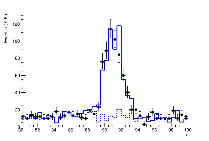
Make an extended probability density function for a distribution in \(m_{\gamma\gamma}\)
An extended probability density model is a product of a probability density function \(f(x)\) in a continuous observable \(x\) and a Poisson model modeling the observed event count \(P(N_\mathrm{obs}|N_\mathrm{exp})\)
For composite pdfs (a sum of 2 of more components) the conceptual expression
can be elegantly rewritten in the producy of a probability density function and Poisson
In [1]:
RooWorkspace w("w") ;
RooFit v3.60 -- Developed by Wouter Verkerke and David Kirkby
Copyright (C) 2000-2013 NIKHEF, University of California & Stanford University
All rights reserved, please read http://roofit.sourceforge.net/license.txt
Exponential distribution for the background and Gaussian distribution for the signal
In [2]:
w.factory("Exponential::bkg(mgg[40,400],alpha[-0.01,-10,0])") ;
w.factory("Gaussian::sig(mgg,mean[125,80,400],width[3,1,10])") ;
Fix signal shape for now
In [3]:
w.var("mean")->setConstant(true) ;
w.var("width")->setConstant(true) ;
Model is sum of signal and background
In [4]:
w.factory("expr::S('mu*Snom',mu[1,-3,6],Snom[50])") ;
w.factory("SUM::model(S*sig,Bnom[10000]*bkg)") ;
Sample a toy unbinned toy dataset from the model If no event count is given, the predicted count of the model is taken (in this case S+B)
In [5]:
RooDataSet* data = w.pdf("model")->generate(*w.var("mgg")) ;
Fit model to toy data - the extended option forces the inclusion of the Poisson term in the likelihood construction
In [6]:
RooFitResult* r = w.pdf("model")->fitTo(*data,RooFit::Save(),RooFit::Extended()) ;
[#1] INFO:Minization -- createNLL: caching constraint set under name CONSTR_OF_PDF_model_FOR_OBS_mgg with 0 entries
[#1] INFO:Minization -- RooMinimizer::optimizeConst: activating const optimization
[#1] INFO:Minization -- The following expressions have been identified as constant and will be precalculated and cached: (sig)
[#1] INFO:Minization -- The following expressions will be evaluated in cache-and-track mode: (bkg)
**********
** 1 **SET PRINT 1
**********
**********
** 2 **SET NOGRAD
**********
PARAMETER DEFINITIONS:
NO. NAME VALUE STEP SIZE LIMITS
1 alpha -1.00000e-02 5.00000e-03 -1.00000e+01 0.00000e+00
2 mu 1.00000e+00 9.00000e-01 -3.00000e+00 6.00000e+00
**********
** 3 **SET ERR 0.5
**********
**********
** 4 **SET PRINT 1
**********
**********
** 5 **SET STR 1
**********
NOW USING STRATEGY 1: TRY TO BALANCE SPEED AGAINST RELIABILITY
**********
** 6 **MIGRAD 1000 1
**********
FIRST CALL TO USER FUNCTION AT NEW START POINT, WITH IFLAG=4.
START MIGRAD MINIMIZATION. STRATEGY 1. CONVERGENCE WHEN EDM .LT. 1.00e-03
FCN=-27531.8 FROM MIGRAD STATUS=INITIATE 10 CALLS 11 TOTAL
EDM= unknown STRATEGY= 1 NO ERROR MATRIX
EXT PARAMETER CURRENT GUESS STEP FIRST
NO. NAME VALUE ERROR SIZE DERIVATIVE
1 alpha -1.00000e-02 5.00000e-03 1.63770e-02 -1.52597e+01
2 mu 1.00000e+00 9.00000e-01 2.02684e-01 -2.10238e+00
ERR DEF= 0.5
MIGRAD MINIMIZATION HAS CONVERGED.
MIGRAD WILL VERIFY CONVERGENCE AND ERROR MATRIX.
COVARIANCE MATRIX CALCULATED SUCCESSFULLY
FCN=-27531.8 FROM MIGRAD STATUS=CONVERGED 27 CALLS 28 TOTAL
EDM=9.49644e-06 STRATEGY= 1 ERROR MATRIX ACCURATE
EXT PARAMETER STEP FIRST
NO. NAME VALUE ERROR SIZE DERIVATIVE
1 alpha -9.99923e-03 1.26457e-04 4.58294e-05 -6.74097e+00
2 mu 1.09775e+00 4.59302e-01 1.16765e-02 -1.41907e-02
ERR DEF= 0.5
EXTERNAL ERROR MATRIX. NDIM= 25 NPAR= 2 ERR DEF=0.5
1.599e-08 7.395e-07
7.395e-07 2.117e-01
PARAMETER CORRELATION COEFFICIENTS
NO. GLOBAL 1 2
1 0.01271 1.000 0.013
2 0.01271 0.013 1.000
**********
** 7 **SET ERR 0.5
**********
**********
** 8 **SET PRINT 1
**********
**********
** 9 **HESSE 1000
**********
COVARIANCE MATRIX CALCULATED SUCCESSFULLY
FCN=-27531.8 FROM HESSE STATUS=OK 10 CALLS 38 TOTAL
EDM=9.49203e-06 STRATEGY= 1 ERROR MATRIX ACCURATE
EXT PARAMETER INTERNAL INTERNAL
NO. NAME VALUE ERROR STEP SIZE VALUE
1 alpha -9.99923e-03 1.26456e-04 9.16588e-06 1.50754e+00
2 mu 1.09775e+00 4.59294e-01 4.67062e-04 -8.95073e-02
ERR DEF= 0.5
EXTERNAL ERROR MATRIX. NDIM= 25 NPAR= 2 ERR DEF=0.5
1.599e-08 7.372e-07
7.372e-07 2.117e-01
PARAMETER CORRELATION COEFFICIENTS
NO. GLOBAL 1 2
1 0.01267 1.000 0.013
2 0.01267 0.013 1.000
[#1] INFO:Minization -- RooMinimizer::optimizeConst: deactivating const optimization
Visualize result
In [7]:
TCanvas* c1 = new TCanvas();
RooPlot* frame = w.var("mgg")->frame() ;
data->plotOn(frame) ;
When plotting an extended pdf you can choose to follow intrinsic prediction for the event count, rather than normalizing the plot to the observed data
To do so request a normalization scale factor 1.0 w.r.t the intrinsic expecation
In [8]:
w.pdf("model")->plotOn(frame,RooFit::Normalization(1.0,RooAbsReal::RelativeExpected)) ;
You can also highlight components of the fit as follows
In [9]:
w.pdf("model")->plotOn(frame,RooFit::Normalization(1.0,RooAbsReal::RelativeExpected),RooFit::Components("bkg"),RooFit::LineStyle(kDashed)) ;
frame->Draw() ;
c1->Draw() ;

[#1] INFO:Plotting -- RooAbsPdf::plotOn(model) directly selected PDF components: (bkg)
[#1] INFO:Plotting -- RooAbsPdf::plotOn(model) indirectly selected PDF components: ()
Now save the workspace with the data a modelconfig so that you can use RooStats to extract limits
Save the generated data as the ‘observed data’
In [10]:
w.import(*data,RooFit::Rename("observed_data")) ;
[#1] INFO:ObjectHandling -- RooWorkspace::import(w) importing dataset modelData
[#1] INFO:ObjectHandling -- RooWorkSpace::import(w) changing name of dataset from modelData to observed_data
Create an empty ModelConfig
In [11]:
RooStats::ModelConfig mc("ModelConfig",&w);
Define the pdf, the parameter of interest and the observables
In [12]:
mc.SetPdf(*w.pdf("model"));
mc.SetParametersOfInterest(*w.var("mu"));
//mc.SetNuisanceParameters(RooArgSet(*w.var("mean"),*w.var("width"),*w.var("alpha")));
mc.SetNuisanceParameters(*w.var("alpha"));
mc.SetObservables(*w.var("mgg"));
Define the current value mu (1) as an hypothesis
In [13]:
w.var("mu")->setVal(1) ;
mc.SetSnapshot(*w.var("mu"));
mc.Print();
=== Using the following for ModelConfig ===
Observables: RooArgSet:: = (mgg)
Parameters of Interest: RooArgSet:: = (mu)
Nuisance Parameters: RooArgSet:: = (alpha)
PDF: RooAddPdf::model[ S * sig + Bnom * bkg ] = 0.110271
Snapshot:
1) 0x7f1a20b9fa80 RooRealVar:: mu = 1 +/- 0.459294 L(-3 - 6) "mu"
import model into the workspace and save to file
In [14]:
w.import(mc);
w.writeToFile("model.root") ;
Build workspace using histogram templates
Build a binned likelihood model version of the ex11 example
- construct a histogram template SH(mgg) with a prediction for the binned signal shape
- construct a histogram template BH(mgg) with a prediction for the binned background shape
- construct a probability model model(mgg) = SH(mgg) + BH(mgg)
This model can be ‘seen’ in two ways
- an extended probability model like ex11 that happen to have binned shapes, i.e.
- model(mγγ) = Nsig/Nsig+Nbkg * pdfSH(mγγ) + Nbkg/Nsig+Nbkg * pdfBH(mγγ)
- \(P(N) = N_\mathrm{sig} + N_\mathrm{bkg}\)
- where pdf_SH,pdf_BH are probability density functions that follow shape of the unit normalized histograms
- A product of Poisson counting experiments for each bin
- model(vec_N) = Product(i=0..n-1) Poisson(N_i | S_i + B_i)
- where N_i i=0…N-1 == vec_N are the observed event counts in each bin and S_i and B_i are the predicted signal and background rate in each bin
Both representations are mathematically equivalent, but expression (2) is in practice faster to calculate because it does not require a normalization calculation over pdf_SH and pdf_BH to happen. While for this very simple example it does not make a noticable difference because the normalization does not depend on any model parameters in scenarios where it does it will effectivelt double the calculation time
Construct simulation workspace to generate template histograms
In [1]:
RooWorkspace wsim("wsim") ;
RooFit v3.60 -- Developed by Wouter Verkerke and David Kirkby
Copyright (C) 2000-2013 NIKHEF, University of California & Stanford University
All rights reserved, please read http://roofit.sourceforge.net/license.txt
Generate two distributions, exponential distribution for the background, Gaussian distribution for the signal
In [2]:
wsim.factory("Exponential::bkg(mgg[40,400],alpha[-0.01,-10,0])") ;
wsim.factory("Gaussian::sig(mgg,mean[125,80,400],width[3,1,10])") ;
RooDataHist* hist_sig = wsim.pdf("sig")->generateBinned(*wsim.var("mgg"),50) ;
RooDataHist* hist_bkg = wsim.pdf("bkg")->generateBinned(*wsim.var("mgg"),10000) ;
Mock data distribution with mu=1.5
In [3]:
wsim.factory("expr::S('mu*Snom',mu[1.5],Snom[50])") ;
wsim.factory("SUM::model(S*sig,Bnom[10000]*bkg)") ;
Given that the sum is an extended model, no speficiation of the event count is needed
In [4]:
RooDataHist* hist_data = wsim.pdf("model")->generateBinned(*wsim.var("mgg")) ;
In [5]:
RooWorkspace w("w") ;
First Import template and mock data histograms
In [6]:
w.import(*hist_sig,RooFit::Rename("template_sig")) ;
w.import(*hist_bkg,RooFit::Rename("template_bkg")) ;
w.import(*hist_data,RooFit::Rename("observed_data")) ;
[#1] INFO:ObjectHandling -- RooWorkspace::import(w) importing dataset genData
[#1] INFO:ObjectHandling -- RooWorkSpace::import(w) changing name of dataset from genData to template_sig
[#1] INFO:ObjectHandling -- RooWorkspace::import(w) importing RooRealVar::mgg
[#1] INFO:ObjectHandling -- RooWorkspace::import(w) importing dataset genData
[#1] INFO:ObjectHandling -- RooWorkSpace::import(w) changing name of dataset from genData to template_bkg
[#1] INFO:ObjectHandling -- RooWorkspace::import(w) importing dataset genData
[#1] INFO:ObjectHandling -- RooWorkSpace::import(w) changing name of dataset from genData to observed_data
Now build signal and background models
Note that we build functions here and not pdfs
In [7]:
w.factory("HistFunc::sig(mgg,template_sig)") ;
w.factory("HistFunc::bkg(mgg,template_bkg)") ;
[#1] INFO:ObjectHandling -- RooWorkspace::import(w) importing dataset template_sig
[#1] INFO:ObjectHandling -- RooWorkspace::import(w) importing dataset template_bkg
Also not that we don’t need to declare mgg here, its definition was imported when we imported the histograms
Now construct a ‘amplitude sum’ probability model, defined asa
scaling the predictions of the template histograms. If the template histograms encode the nominal event yield, one expects both coefficients to fit to 1 if the data matches the prediction
NOTE: If the bin width is not equal to one then the event count of a histogram is not identical to the integral over a histogram. In RooFit the **integral* over the histogram is taken as the yield prediction, whereas one usually, interprets the histogram event count as the prediction. The simplest way to correct for this is to multiply \(c_\mathrm{i}\) with a constant which is 1/binwidth*
In this case we choose \(c_\mathrm{sig} = \mu\) (as usual) and introduce a Bscale as a nuisance parameter that can freely scale the background
In [8]:
w.factory("binw[0.277]") ; // == 1/(400-30)
w.factory("expr::S('mu*binw',mu[1,-1,6],binw[0.277])") ;
w.factory("expr::B('Bscale*binw',Bscale[0,6],binw)") ;
w.factory("ASUM::model(S*sig,B*bkg)") ;
[#1] INFO:ObjectHandling -- RooWorkSpace::import(w) Recycling existing object binw created with identical factory specification
Fit the binned probability model to the binned data
In [9]:
w.pdf("model")->fitTo(*hist_data) ;
TCanvas* c1 = new TCanvas();
RooPlot* frame = w.var("mgg")->frame() ;
hist_data->plotOn(frame) ;
w.pdf("model")->plotOn(frame) ;
w.pdf("model")->plotOn(frame,RooFit::Components("bkg"),RooFit::LineStyle(kDashed)) ;
frame->Draw() ;
c1->Draw();
[#1] INFO:Minization -- p.d.f. provides expected number of events, including extended term in likelihood.
[#1] INFO:Minization -- createNLL: caching constraint set under name CONSTR_OF_PDF_model_FOR_OBS_mgg with 0 entries
[#1] INFO:Minization -- RooMinimizer::optimizeConst: activating const optimization
[#1] INFO:Minization -- The following expressions have been identified as constant and will be precalculated and cached: (sig,bkg)
**********
** 1 **SET PRINT 1
**********
**********
** 2 **SET NOGRAD
**********
PARAMETER DEFINITIONS:
NO. NAME VALUE STEP SIZE LIMITS
1 Bscale 3.00000e+00 6.00000e-01 0.00000e+00 6.00000e+00
2 mu 1.00000e+00 7.00000e-01 -1.00000e+00 6.00000e+00
**********
** 3 **SET ERR 0.5
**********
**********
** 4 **SET PRINT 1
**********
**********
** 5 **SET STR 1
**********
NOW USING STRATEGY 1: TRY TO BALANCE SPEED AGAINST RELIABILITY
**********
** 6 **MIGRAD 1000 1
**********
FIRST CALL TO USER FUNCTION AT NEW START POINT, WITH IFLAG=4.
START MIGRAD MINIMIZATION. STRATEGY 1. CONVERGENCE WHEN EDM .LT. 1.00e-03
FCN=-18731 FROM MIGRAD STATUS=INITIATE 6 CALLS 7 TOTAL
EDM= unknown STRATEGY= 1 NO ERROR MATRIX
EXT PARAMETER CURRENT GUESS STEP FIRST
NO. NAME VALUE ERROR SIZE DERIVATIVE
1 Bscale 3.00000e+00 6.00000e-01 2.01358e-01 1.98597e+04
2 mu 1.00000e+00 7.00000e-01 2.24553e-01 9.86124e+01
ERR DEF= 0.5
MIGRAD MINIMIZATION HAS CONVERGED.
MIGRAD WILL VERIFY CONVERGENCE AND ERROR MATRIX.
COVARIANCE MATRIX CALCULATED SUCCESSFULLY
FCN=-27643.4 FROM MIGRAD STATUS=CONVERGED 63 CALLS 64 TOTAL
EDM=1.90326e-05 STRATEGY= 1 ERROR MATRIX ACCURATE
EXT PARAMETER STEP FIRST
NO. NAME VALUE ERROR SIZE DERIVATIVE
1 Bscale 1.00258e+00 1.02810e-02 5.15767e-04 -9.00358e-01
2 mu 1.54130e+00 4.86712e-01 1.62486e-02 -1.71092e-02
ERR DEF= 0.5
EXTERNAL ERROR MATRIX. NDIM= 25 NPAR= 2 ERR DEF=0.5
1.057e-04 -1.035e-03
-1.035e-03 2.386e-01
PARAMETER CORRELATION COEFFICIENTS
NO. GLOBAL 1 2
1 0.20612 1.000 -0.206
2 0.20612 -0.206 1.000
**********
** 7 **SET ERR 0.5
**********
**********
** 8 **SET PRINT 1
**********
**********
** 9 **HESSE 1000
**********
COVARIANCE MATRIX CALCULATED SUCCESSFULLY
FCN=-27643.4 FROM HESSE STATUS=OK 10 CALLS 74 TOTAL
EDM=1.90282e-05 STRATEGY= 1 ERROR MATRIX ACCURATE
EXT PARAMETER INTERNAL INTERNAL
NO. NAME VALUE ERROR STEP SIZE VALUE
1 Bscale 1.00258e+00 1.02822e-02 1.03153e-04 -7.28574e-01
2 mu 1.54130e+00 4.86745e-01 3.24972e-03 -2.77461e-01
ERR DEF= 0.5
EXTERNAL ERROR MATRIX. NDIM= 25 NPAR= 2 ERR DEF=0.5
1.057e-04 -1.038e-03
-1.038e-03 2.386e-01
PARAMETER CORRELATION COEFFICIENTS
NO. GLOBAL 1 2
1 0.20664 1.000 -0.207
2 0.20664 -0.207 1.000
[#1] INFO:Minization -- RooMinimizer::optimizeConst: deactivating const optimization
[#1] INFO:Plotting -- RooAbsPdf::plotOn(model) directly selected PDF components: (bkg)
[#1] INFO:Plotting -- RooAbsPdf::plotOn(model) indirectly selected PDF components: ()

Now save the workspace with the data a modelconfig so that you can use RooStats to extract limits
Create an empty ModelConfig
In [10]:
RooStats::ModelConfig mc("ModelConfig",&w);
Define the pdf, the parameter of interest and the observables
In [11]:
mc.SetPdf(*w.pdf("model"));
mc.SetParametersOfInterest(*w.var("mu"));
//mc.SetNuisanceParameters(RooArgSet(*w.var("mean"),*w.var("width"),*w.var("alpha")));
mc.SetNuisanceParameters(*w.var("Bscale"));
mc.SetObservables(*w.var("mgg"));
Define the current value \(\mu=1\) as an hypothesis
In [12]:
w.var("mu")->setVal(1) ;
mc.SetSnapshot(*w.var("mu"));
mc.Print();
=== Using the following for ModelConfig ===
Observables: RooArgSet:: = (mgg)
Parameters of Interest: RooArgSet:: = (mu)
Nuisance Parameters: RooArgSet:: = (Bscale)
PDF: RooRealSumPdf::model[ S * sig + B * bkg ] = 2.77715
Snapshot:
1) 0x7fe4dca0cd80 RooRealVar:: mu = 1 +/- 0.486745 L(-1 - 6) "mu"
import model in the workspace
In [13]:
w.import(mc);
w.writeToFile("model.root") ;
A couple of final important points on RooFit models and workspace
- The factory is an efficient way to quickly express what RooFit objects should be instantiated. Objects built with the factory
are not in any way different from those created ‘manually’ and then imported into the workspace.
- All objects (wether created through the factory or imported) can be modified a posteriori, e.g. modification of advanced
settings from class methods, after they have been created and/or imported. All such changes in settings are persisted with the workspace. The factory does therefore on purpose not provide an interface for such modifications.
- All RooFit objects in a workspace should have unique names. The factory and import methods automatically enforce this
Building joint models and data structures
the general case
When building joint probability models for multiple datasets, e.g. simultaneous fits or profile likelihood models in general, there are some important point to consider when building the model. In the RooFit paradigm such joint fits are best constructed by first joining all independent datasets together into a single composite ‘master’ dataset, and by joining all probability models corresponding to the individual datasets into a composite ‘master’ probability model. If it is done this way, all main statistical operations ranging from basic operations like fitting and toy data generation to advanced limit setting procedures work on composite models with exactly the same interface as for simple models. This design choices greatly simplifies the syntax of the high level statistical tools, but introduces some additional syntax to express composite datasets and probability models, which are discussion in this section.
Joining probability models for disjoint datasets
A joint probability model that simultaneously describes two or more disjoint datasets is represented in RooFit by class RooSimultaneous, which is constructed in the factory with the SIMUL operator:
// Construct joint model for signal region and a control region
// This example assumes a pdf sigModel and ctlModel were previously defined
// in the workspace (the internal structure of these models is irrelevant)
//
w.factory("SIMUL::master(index[SIG,CTL],SIG=sigModel,CTL=ctlModel)") ;
The code above generates two new objects
- A new discrete observable (class RooCategory) named ‘index’ that has two defined states: SIG and CTL that serves
as additional observable to the newly create pdf master (in addition to the observables defined in sigModel and ctlModel). The role of this observable is to indicate which component pdf should be used to interpret the remaining observables in the dataset
- A new joint probability model master that describes both distributions. Suppose sigModel describes the distribution
of observable x and ctlModel describes the distribution of observable y, then the observables of the joint model are {index, x, y}
Joining disjoint datasets into a master dataset
The joint dataset that is needed to construct a likelihood from ‘master’ model must thus also conform to this structure: it’s observable must include both x and y, as well as the discrete index variable to label to which component dataset each event belongs. It is instructive to first consider visually what this data organization entails
D(x) D(y) D(index,x,y)
1.5 23 SIG, 1.5, -
2.3 17 —> SIG, 2.3, -
4.7 98 SIG, 4.7, -
CTL, - , 23
CTL, - , 17
CTL, - , 98
The joining of datasets is trivially perform in the RooDataSet constructor
// The example assume this existence of a workspace that defines variable, x,y,index
// Construct a dataset D(x)
RooDataSet d_sig("d_sig","d_sig",*w.var("x")) ;
w.var("x")->setValue(1.5) ;
d_sig.add(*w.var("x")) ; // fill data, etc..
// Construct a dataset D(y)
RooDataSet d_ctl("d_ctl","d_ctl",*w.var("y")) ;
w.var("y")->setValue(23) ;
d_ctl.add(*w.var("xy")) ; // fill data, etc..
// Construct a joint dataset D(index,x,y)
map<string,RooDataSet*> dmap;
dmap["SIG"]=&d_sig ;
dmap["CTL"]=&d_ctl ;
RooDataSet d_joint("d_joint","d_joint",Index(*w.cat("index")),Import(dmap)) ;
Note that while a composite RooDataSet externally presents the interface of a simple dataset with observables (index,x,y) it is internally organised in subdatasets for efficient storage and data retrieval
D(index,x,y) D(index,x,y)
SIG, 1.5, - index==SIG index==CTL
SIG, 2.3, - D(x) D(y)
SIG, 4.7, - —> 1.5 23
CTL, - , 23 2.3 17
CTL, - , 17 4.7 98
CTL, - , 98
This internal data organization is also introduced for toy data sets that are sampled from composite datasets.
Working with joint models and datasets
Once the joint model master(index,x,y) and a joint dataset D(index,x,y) are constructed, all operations work exactly as for simple models. For example, a joint fit is trivially performed as follows
w.pdf("master")->fitTo(d_joint) ;
An important part of the design of joint models is that there is no performance loss due to computation overhead in the joint construction: when the joint likelihood is constructed from a joint model and dataset, it is internally organised again in component likelihoods, where each component model of master is match to the corresponding component dataset of d_joint, and subsequently separately optimised for computational efficiency.
profile likelihood models & global observables
While the interface described in the previous sections works for joint models of any shape and form, a dedicated syntax exists for the formulation of so-called ‘profile likelihood’ models. The key difference between a generic joint model and a ‘profile likelihood’ joint model is that in the latter the internal structure of the control region (now named ‘subsidiary measurement’ is simplified to a Gaussian, Poisson or LogNormal distribution so that the corresponding observation can be represented by a single number, where the convention of the subsidiary measurement is furthermore chosen such, through a suitable transformation of the meaning of the parameters, that the observed values is either always zero or one
Such likelihood can in principle be described with a joint dataset \(D`(index,:math:`x_\mathrm{sig}\),0,0,….0) and a corresponding SIMUL probability model with equally many components, but the carrying around of hundreds of observed values that are always identical to zero can be cumbersome.
Hence an alternative formulation style exists in RooFit that is specifically suitable for profile likelihood models - here the observed value of the subsidiary measurements is simply encoded in observable variable of the pdf itself, rather than in an external dataset. Hence instead of a dataset/model pair in traditional joint format
one writes
where the observable \(y_\mathrm{ctl}==0\) is dropped from the dataset, as well as the index observable, as it is no longer needed to distinguish between data belonging to the main measurement and the subsidiary measurement(s). This greatly simplifies the formulation of datasets of profile likelihood models. On the probability model side, the formulation then changes as follows
- Instead of using
SIMUL()to multiply subsidiary measurements with the main measurement, thePROD()operator
is used, which does not require the introduction of an index observable to label events
- The model variables that represent the subsidiary measurements must be explicitly labeled in the object as such
(to distinguish these from parameters). This can be either done intrinsically in the model, or this specification can be provided externally when an operation (fit, toyMC generation etc) is performed
In the LHC jargon the variables in the model that represent the (trivial) values of the observables of the subsidiary measurements are named the “Global Observables”. The easiest-to-use way to mark global observables in the model is to label them as such
// repeat for each global observable
w.var(“obs_alpha”)->setAttribute(“MyGlobalObservable”) ;
// advertise string label used to mark global observables in the top-level pdf object
w.pdf(“master”)->setStringAttribute(“GlobalObservablesTag”,”MyGlobalObservable”) ;
Most modeling building tools currently in use, do not yet take advantage to label these observables as such in the model.
Instead it is common practice, to specify these always external through a GlobalObservables() command-line specification when fitting or generation.
To simplify this external specification process for RooStats tools, the ModelConfig interface object allows the global observables to
be specified there, so that its definition is always consistently used by all RooStats tools.
// Define the pdf, the parameter of interest and the observables
mc.SetPdf(*w.pdf(“p"));
mc.SetParametersOfInterest(*w.var("mu"));
mc.SetGlobalObservables(…..);
mc.SetObservables(*w.var(“n"));
Any code that works with profile likelihood that wishes this external specification of the global observables, in addition to the internal specifications must incorporate some explicit handling of thus. Here is a modified version of the run_fit() macro of the previous section that does so
void run_fit(const char* workspaceName, const char* datasetName) {
// Reviving a model from a workspace
TFile* f = TFile::Open("model.root") ;
RooWorkspace* w = (RooWorkspace*) f->Get("w") ;
RooStats:::ModelConfig* mc = (RooStats::ModelConfig*) w->genobj("ModelConfig") ;
RooAbsPdf* pdf = w->pdf(mc->GetPdf()->GetName()) ;
RooArgSet* globs = mc->GetGlobalObservables() ;
// Load data from workspace
RooAbsData* data = w->data(datasetName) ;
if (!pdf || !data) return ;
if (globs) {
pdf->fitTo(*data, GlobalObservables(*globs)) ;
} else {
pdf->fitTo(*data)
}
|
def run_fit(workspaceName, datasetName):
# Reviving a model from a workspace
f = ROOT.TFile.Open("model.root")
w = f.Get(workspaceName)
mc = w.genobj("ModelConfig")
pdf = w.pdf(mc.GetPdf().GetName())
globs = mc.GetGlobalObservables()
# Load data from workspace
data = w.data(datasetName)
if pdf is None or data is None: return None
if globs:
pdf.fitTo(data, ROOT.RooFit.GlobalObservables(globs))
else:
pdf.fitTo(data)
|
The processing of intrinsic global variable specifications is always automatic, but unfortunately it’s use is not common practice yet in LHC models.
Tools for model building and model manipulation
List of available tools [ Combiners, HistFactory, HistFitter, etc… ]
HistFactory
A histfactory model is built as follows
- A channel is modeled by a stack of samples (signal, backgrounds)
- A measurement is composed of one or more channels
In [1]:
using namespace RooStats;
using namespace HistFactory;
Create the measurement
In [2]:
std::string inputFileName = "./input/example.root";
HistFactory::Measurement meas("meas", "meas");
meas.SetOutputFilePrefix( "./results/example_" );
RooFit v3.60 -- Developed by Wouter Verkerke and David Kirkby
Copyright (C) 2000-2013 NIKHEF, University of California & Stanford University
All rights reserved, please read http://roofit.sourceforge.net/license.txt
Define the name of the POI
In [3]:
meas.SetPOI("mu");
Declare constants
In [4]:
meas.AddConstantParam("alpha_syst1");
meas.AddConstantParam("Lumi");
Set luminosity and its uncertainty
In [5]:
meas.SetLumi(1.0);
meas.SetLumiRelErr(0.10);
…and some technical configuration…
In [6]:
meas.SetExportOnly(false);
meas.SetBinHigh(2);
Create a channel
In [7]:
HistFactory::Channel chan("channel1");
chan.SetData("data",inputFileName) ;
chan.SetStatErrorConfig(0.05, "Poisson");
Populate this channel with samples
Signal sample - scaled by a normalization factor \(\mu\) and
with a 5% systematic scale uncertainty named syst1
In [8]:
HistFactory::Sample sig( "signal", "signal", inputFileName ) ;
sig.AddOverallSys("syst1",0.95,1.05) ;
sig.AddNormFactor("mu",1,0,3 ) ;
chan.AddSample(sig) ;
Background sample 1 - with a 5% systematic scale uncertainty named syst2 and with modeling of MC statistical, uncertainties
In [9]:
HistFactory::Sample background1("background1","background1",inputFileName) ;
background1.ActivateStatError("background1_statUncert",inputFileName) ;
background1.AddOverallSys("syst2",0.95,1.05) ;
chan.AddSample(background1) ;
Background sample 2 - with a 5% systematic scale uncertainty named syst3 - and with modeling of MC statistical uncertainties
In [10]:
HistFactory::Sample background2( "background2", "background2", inputFileName );
background2.ActivateStatError();
background2.AddOverallSys("syst3",0.95,1.05);
chan.AddSample( background2) ;
Add channel to the measurementa
In [11]:
meas.AddChannel( chan );
Collect all the required templated histograms from the input file
In [12]:
meas.CollectHistograms();
Getting histogram. InputFile ./input/example.root HistoPath HistoName data
Opened input file: ./input/example.root: 0x7f507c3030f0
Collecting Nominal Histogram
Getting histogram. InputFile ./input/example.root HistoPath HistoName signal
Opened input file: ./input/example.root: 0x7f507c510350
Collecting Nominal Histogram
Getting histogram. InputFile ./input/example.root HistoPath HistoName background1
Opened input file: ./input/example.root: 0x7f507c419120
Getting histogram. InputFile ./input/example.root HistoPath HistoName background1_statUncert
Opened input file: ./input/example.root: 0x7f507c5111b0
Collecting Nominal Histogram
Getting histogram. InputFile ./input/example.root HistoPath HistoName background2
Opened input file: ./input/example.root: 0x7f507c53c950
Now build a workspace with a pdf and a modelconfig
In [13]:
RooWorkspace* w = MakeModelAndMeasurementFast(meas) ;
Making Model and Measurements (Fast) for measurement: meas
using lumi = 1 and lumiError = 0.1 including bins between 0 and 2
fixing the following parameters:
alpha_syst1
Lumi
Checking if output directory : ./results - exists
Creating the output file: ./results/example__meas.root
Creating the table file: ./results/example__results.table
Creating the HistoToWorkspaceFactoryFast factory
Setting preprocess functions
Starting to process channel: channel1
-------------------
Starting to process channel1 channel with 1 observables
lumi str = [1,0,10]
lumi Error str = nominalLumi[1,0,2],0.1
[#1] INFO:ObjectHandling -- RooWorkspace::import(channel1) importing RooStats::HistFactory::FlexibleInterpVar::signal_channel1_epsilon
making normFactor: mu
signal_channel1 has no variation histograms
processing hist signal
[#1] INFO:DataHandling -- RooDataHist::adjustBinning(signal_channel1nominalDHist): fit range of variable obs_x_channel1 expanded to nearest bin boundaries: [1,2] --> [1,2]
[#1] INFO:ObjectHandling -- RooWorkspace::import(channel1) importing dataset signal_channel1nominalDHist
[#1] INFO:ObjectHandling -- RooWorkspace::import(channel1) importing RooHistFunc::signal_channel1_nominal
[#1] INFO:ObjectHandling -- RooWorkspace::import(channel1) importing RooStats::HistFactory::FlexibleInterpVar::background1_channel1_epsilon
background1_channel1 has no variation histograms
processing hist background1
[#1] INFO:DataHandling -- RooDataHist::adjustBinning(background1_channel1nominalDHist): fit range of variable obs_x_channel1 expanded to nearest bin boundaries: [1,2] --> [1,2]
[#1] INFO:ObjectHandling -- RooWorkspace::import(channel1) importing dataset background1_channel1nominalDHist
[#1] INFO:ObjectHandling -- RooWorkspace::import(channel1) importing RooHistFunc::background1_channel1_nominal
Sample: background1 to be included in Stat Error for channel channel1
Using external histogram for Stat Errors for Channel: channel1 Sample: background1
Error Histogram: background1_statUncert
[#1] INFO:ObjectHandling -- RooWorkspace::import(channel1) importing RooRealVar::gamma_stat_channel1_bin_0
[#1] INFO:ObjectHandling -- RooWorkspace::import(channel1) importing RooRealVar::gamma_stat_channel1_bin_1
[#1] INFO:ObjectHandling -- RooWorkspace::import(channel1) importing ParamHistFunc::mc_stat_channel1
[#1] INFO:ObjectHandling -- RooWorkspace::import(channel1) using existing copy of RooRealVar::obs_x_channel1 for import of ParamHistFunc::mc_stat_channel1
[#1] INFO:ObjectHandling -- RooWorkspace::import(channel1) using existing copy of RooRealVar::gamma_stat_channel1_bin_0 for import of ParamHistFunc::mc_stat_channel1
[#1] INFO:ObjectHandling -- RooWorkspace::import(channel1) using existing copy of RooRealVar::gamma_stat_channel1_bin_1 for import of ParamHistFunc::mc_stat_channel1
[#1] INFO:ObjectHandling -- RooWorkspace::import(channel1) importing RooProduct::background1_channel1_overallSyst_x_StatUncert
[#1] INFO:ObjectHandling -- RooWorkspace::import(channel1) using existing copy of ParamHistFunc::mc_stat_channel1 for import of RooProduct::background1_channel1_overallSyst_x_StatUncert
[#1] INFO:ObjectHandling -- RooWorkspace::import(channel1) using existing copy of RooRealVar::obs_x_channel1 for import of RooProduct::background1_channel1_overallSyst_x_StatUncert
[#1] INFO:ObjectHandling -- RooWorkspace::import(channel1) using existing copy of RooRealVar::gamma_stat_channel1_bin_0 for import of RooProduct::background1_channel1_overallSyst_x_StatUncert
[#1] INFO:ObjectHandling -- RooWorkspace::import(channel1) using existing copy of RooRealVar::gamma_stat_channel1_bin_1 for import of RooProduct::background1_channel1_overallSyst_x_StatUncert
[#1] INFO:ObjectHandling -- RooWorkspace::import(channel1) using existing copy of RooProduct::background1_channel1_overallSyst_x_Exp for import of RooProduct::background1_channel1_overallSyst_x_StatUncert
[#1] INFO:ObjectHandling -- RooWorkspace::import(channel1) using existing copy of RooHistFunc::background1_channel1_nominal for import of RooProduct::background1_channel1_overallSyst_x_StatUncert
[#1] INFO:ObjectHandling -- RooWorkspace::import(channel1) using existing copy of RooStats::HistFactory::FlexibleInterpVar::background1_channel1_epsilon for import of RooProduct::background1_channel1_overallSyst_x_StatUncert
[#1] INFO:ObjectHandling -- RooWorkspace::import(channel1) using existing copy of RooRealVar::alpha_syst2 for import of RooProduct::background1_channel1_overallSyst_x_StatUncert
[#1] INFO:ObjectHandling -- RooWorkspace::import(channel1) importing RooStats::HistFactory::FlexibleInterpVar::background2_channel1_epsilon
background2_channel1 has no variation histograms
processing hist background2
[#1] INFO:DataHandling -- RooDataHist::adjustBinning(background2_channel1nominalDHist): fit range of variable obs_x_channel1 expanded to nearest bin boundaries: [1,2] --> [1,2]
[#1] INFO:ObjectHandling -- RooWorkspace::import(channel1) importing dataset background2_channel1nominalDHist
[#1] INFO:ObjectHandling -- RooWorkspace::import(channel1) importing RooHistFunc::background2_channel1_nominal
Sample: background2 to be included in Stat Error for channel channel1
Making Statistical Uncertainty Hist for Channel: channel1 Sample: background2
[#1] INFO:ObjectHandling -- RooWorkspace::import(channel1) importing RooProduct::background2_channel1_overallSyst_x_StatUncert
[#1] INFO:ObjectHandling -- RooWorkspace::import(channel1) using existing copy of ParamHistFunc::mc_stat_channel1 for import of RooProduct::background2_channel1_overallSyst_x_StatUncert
[#1] INFO:ObjectHandling -- RooWorkspace::import(channel1) using existing copy of RooRealVar::obs_x_channel1 for import of RooProduct::background2_channel1_overallSyst_x_StatUncert
[#1] INFO:ObjectHandling -- RooWorkspace::import(channel1) using existing copy of RooRealVar::gamma_stat_channel1_bin_0 for import of RooProduct::background2_channel1_overallSyst_x_StatUncert
[#1] INFO:ObjectHandling -- RooWorkspace::import(channel1) using existing copy of RooRealVar::gamma_stat_channel1_bin_1 for import of RooProduct::background2_channel1_overallSyst_x_StatUncert
[#1] INFO:ObjectHandling -- RooWorkspace::import(channel1) using existing copy of RooProduct::background2_channel1_overallSyst_x_Exp for import of RooProduct::background2_channel1_overallSyst_x_StatUncert
[#1] INFO:ObjectHandling -- RooWorkspace::import(channel1) using existing copy of RooHistFunc::background2_channel1_nominal for import of RooProduct::background2_channel1_overallSyst_x_StatUncert
[#1] INFO:ObjectHandling -- RooWorkspace::import(channel1) using existing copy of RooStats::HistFactory::FlexibleInterpVar::background2_channel1_epsilon for import of RooProduct::background2_channel1_overallSyst_x_StatUncert
[#1] INFO:ObjectHandling -- RooWorkspace::import(channel1) using existing copy of RooRealVar::alpha_syst3 for import of RooProduct::background2_channel1_overallSyst_x_StatUncert
Making Total Uncertainty for bin 1 Error = 5 Val = 100 RelativeError = 0.05
Making Total Uncertainty for bin 2 Error = 10 Val = 100 RelativeError = 0.1
About to create Constraint Terms from: mc_stat_channel1 params: (gamma_stat_channel1_bin_0,gamma_stat_channel1_bin_1)
Using Poisson StatErrors in channel: channel1
Creating constraint for: gamma_stat_channel1_bin_0. Type of constraint: 1
[#1] INFO:ObjectHandling -- RooWorkspace::import(channel1) importing RooPoisson::gamma_stat_channel1_bin_0_constraint
[#1] INFO:ObjectHandling -- RooWorkspace::import(channel1) importing RooRealVar::nom_gamma_stat_channel1_bin_0
[#1] INFO:ObjectHandling -- RooWorkspace::import(channel1) importing RooProduct::gamma_stat_channel1_bin_0_poisMean
[#1] INFO:ObjectHandling -- RooWorkspace::import(channel1) using existing copy of RooRealVar::gamma_stat_channel1_bin_0 for import of RooPoisson::gamma_stat_channel1_bin_0_constraint
[#1] INFO:ObjectHandling -- RooWorkspace::import(channel1) importing RooConstVar::gamma_stat_channel1_bin_0_tau
Creating constraint for: gamma_stat_channel1_bin_1. Type of constraint: 1
[#1] INFO:ObjectHandling -- RooWorkspace::import(channel1) importing RooPoisson::gamma_stat_channel1_bin_1_constraint
[#1] INFO:ObjectHandling -- RooWorkspace::import(channel1) importing RooRealVar::nom_gamma_stat_channel1_bin_1
[#1] INFO:ObjectHandling -- RooWorkspace::import(channel1) importing RooProduct::gamma_stat_channel1_bin_1_poisMean
[#1] INFO:ObjectHandling -- RooWorkspace::import(channel1) using existing copy of RooRealVar::gamma_stat_channel1_bin_1 for import of RooPoisson::gamma_stat_channel1_bin_1_constraint
[#1] INFO:ObjectHandling -- RooWorkspace::import(channel1) importing RooConstVar::gamma_stat_channel1_bin_1_tau
[#1] INFO:ObjectHandling -- RooWorkspace::import(channel1) importing RooRealSumPdf::channel1_model
-----------------------------------------
import model into workspace
[#1] INFO:ObjectHandling -- RooWorkspace::import(channel1) importing RooProdPdf::model_channel1
[#1] INFO:ObjectHandling -- RooWorkspace::import(channel1) using existing copy of RooGaussian::lumiConstraint for import of RooProdPdf::model_channel1
[#1] INFO:ObjectHandling -- RooWorkspace::import(channel1) using existing copy of RooConstVar::0.1 for import of RooProdPdf::model_channel1
[#1] INFO:ObjectHandling -- RooWorkspace::import(channel1) using existing copy of RooRealVar::Lumi for import of RooProdPdf::model_channel1
[#1] INFO:ObjectHandling -- RooWorkspace::import(channel1) using existing copy of RooRealVar::nominalLumi for import of RooProdPdf::model_channel1
[#1] INFO:ObjectHandling -- RooWorkspace::import(channel1) using existing copy of RooGaussian::alpha_syst1Constraint for import of RooProdPdf::model_channel1
[#1] INFO:ObjectHandling -- RooWorkspace::import(channel1) using existing copy of RooConstVar::1 for import of RooProdPdf::model_channel1
[#1] INFO:ObjectHandling -- RooWorkspace::import(channel1) using existing copy of RooRealVar::alpha_syst1 for import of RooProdPdf::model_channel1
[#1] INFO:ObjectHandling -- RooWorkspace::import(channel1) using existing copy of RooRealVar::nom_alpha_syst1 for import of RooProdPdf::model_channel1
[#1] INFO:ObjectHandling -- RooWorkspace::import(channel1) using existing copy of RooGaussian::alpha_syst2Constraint for import of RooProdPdf::model_channel1
[#1] INFO:ObjectHandling -- RooWorkspace::import(channel1) using existing copy of RooRealVar::alpha_syst2 for import of RooProdPdf::model_channel1
[#1] INFO:ObjectHandling -- RooWorkspace::import(channel1) using existing copy of RooRealVar::nom_alpha_syst2 for import of RooProdPdf::model_channel1
[#1] INFO:ObjectHandling -- RooWorkspace::import(channel1) using existing copy of RooGaussian::alpha_syst3Constraint for import of RooProdPdf::model_channel1
[#1] INFO:ObjectHandling -- RooWorkspace::import(channel1) using existing copy of RooRealVar::alpha_syst3 for import of RooProdPdf::model_channel1
[#1] INFO:ObjectHandling -- RooWorkspace::import(channel1) using existing copy of RooRealVar::nom_alpha_syst3 for import of RooProdPdf::model_channel1
[#1] INFO:ObjectHandling -- RooWorkspace::import(channel1) using existing copy of RooPoisson::gamma_stat_channel1_bin_0_constraint for import of RooProdPdf::model_channel1
[#1] INFO:ObjectHandling -- RooWorkspace::import(channel1) using existing copy of RooRealVar::nom_gamma_stat_channel1_bin_0 for import of RooProdPdf::model_channel1
[#1] INFO:ObjectHandling -- RooWorkspace::import(channel1) using existing copy of RooProduct::gamma_stat_channel1_bin_0_poisMean for import of RooProdPdf::model_channel1
[#1] INFO:ObjectHandling -- RooWorkspace::import(channel1) using existing copy of RooConstVar::gamma_stat_channel1_bin_0_tau for import of RooProdPdf::model_channel1
[#1] INFO:ObjectHandling -- RooWorkspace::import(channel1) using existing copy of RooRealVar::gamma_stat_channel1_bin_0 for import of RooProdPdf::model_channel1
[#1] INFO:ObjectHandling -- RooWorkspace::import(channel1) using existing copy of RooPoisson::gamma_stat_channel1_bin_1_constraint for import of RooProdPdf::model_channel1
[#1] INFO:ObjectHandling -- RooWorkspace::import(channel1) using existing copy of RooRealVar::nom_gamma_stat_channel1_bin_1 for import of RooProdPdf::model_channel1
[#1] INFO:ObjectHandling -- RooWorkspace::import(channel1) using existing copy of RooProduct::gamma_stat_channel1_bin_1_poisMean for import of RooProdPdf::model_channel1
[#1] INFO:ObjectHandling -- RooWorkspace::import(channel1) using existing copy of RooConstVar::gamma_stat_channel1_bin_1_tau for import of RooProdPdf::model_channel1
[#1] INFO:ObjectHandling -- RooWorkspace::import(channel1) using existing copy of RooRealVar::gamma_stat_channel1_bin_1 for import of RooProdPdf::model_channel1
[#1] INFO:ObjectHandling -- RooWorkspace::import(channel1) using existing copy of RooRealSumPdf::channel1_model for import of RooProdPdf::model_channel1
[#1] INFO:ObjectHandling -- RooWorkspace::import(channel1) using existing copy of RooProduct::L_x_signal_channel1_overallSyst_x_Exp for import of RooProdPdf::model_channel1
[#1] INFO:ObjectHandling -- RooWorkspace::import(channel1) using existing copy of RooProduct::signal_channel1_overallSyst_x_Exp for import of RooProdPdf::model_channel1
[#1] INFO:ObjectHandling -- RooWorkspace::import(channel1) using existing copy of RooHistFunc::signal_channel1_nominal for import of RooProdPdf::model_channel1
[#1] INFO:ObjectHandling -- RooWorkspace::import(channel1) using existing copy of RooRealVar::obs_x_channel1 for import of RooProdPdf::model_channel1
[#1] INFO:ObjectHandling -- RooWorkspace::import(channel1) using existing copy of RooProduct::signal_channel1_overallNorm_x_sigma_epsilon for import of RooProdPdf::model_channel1
[#1] INFO:ObjectHandling -- RooWorkspace::import(channel1) using existing copy of RooRealVar::mu for import of RooProdPdf::model_channel1
[#1] INFO:ObjectHandling -- RooWorkspace::import(channel1) using existing copy of RooStats::HistFactory::FlexibleInterpVar::signal_channel1_epsilon for import of RooProdPdf::model_channel1
[#1] INFO:ObjectHandling -- RooWorkspace::import(channel1) using existing copy of RooRealVar::binWidth_obs_x_channel1_0 for import of RooProdPdf::model_channel1
[#1] INFO:ObjectHandling -- RooWorkspace::import(channel1) using existing copy of RooProduct::L_x_background1_channel1_overallSyst_x_StatUncert for import of RooProdPdf::model_channel1
[#1] INFO:ObjectHandling -- RooWorkspace::import(channel1) using existing copy of RooProduct::background1_channel1_overallSyst_x_StatUncert for import of RooProdPdf::model_channel1
[#1] INFO:ObjectHandling -- RooWorkspace::import(channel1) using existing copy of ParamHistFunc::mc_stat_channel1 for import of RooProdPdf::model_channel1
[#1] INFO:ObjectHandling -- RooWorkspace::import(channel1) using existing copy of RooProduct::background1_channel1_overallSyst_x_Exp for import of RooProdPdf::model_channel1
[#1] INFO:ObjectHandling -- RooWorkspace::import(channel1) using existing copy of RooHistFunc::background1_channel1_nominal for import of RooProdPdf::model_channel1
[#1] INFO:ObjectHandling -- RooWorkspace::import(channel1) using existing copy of RooStats::HistFactory::FlexibleInterpVar::background1_channel1_epsilon for import of RooProdPdf::model_channel1
[#1] INFO:ObjectHandling -- RooWorkspace::import(channel1) using existing copy of RooRealVar::binWidth_obs_x_channel1_1 for import of RooProdPdf::model_channel1
[#1] INFO:ObjectHandling -- RooWorkspace::import(channel1) using existing copy of RooProduct::L_x_background2_channel1_overallSyst_x_StatUncert for import of RooProdPdf::model_channel1
[#1] INFO:ObjectHandling -- RooWorkspace::import(channel1) using existing copy of RooProduct::background2_channel1_overallSyst_x_StatUncert for import of RooProdPdf::model_channel1
[#1] INFO:ObjectHandling -- RooWorkspace::import(channel1) using existing copy of RooProduct::background2_channel1_overallSyst_x_Exp for import of RooProdPdf::model_channel1
[#1] INFO:ObjectHandling -- RooWorkspace::import(channel1) using existing copy of RooHistFunc::background2_channel1_nominal for import of RooProdPdf::model_channel1
[#1] INFO:ObjectHandling -- RooWorkspace::import(channel1) using existing copy of RooStats::HistFactory::FlexibleInterpVar::background2_channel1_epsilon for import of RooProdPdf::model_channel1
[#1] INFO:ObjectHandling -- RooWorkspace::import(channel1) using existing copy of RooRealVar::binWidth_obs_x_channel1_2 for import of RooProdPdf::model_channel1
[#1] INFO:NumericIntegration -- RooRealIntegral::init(channel1_model_Int[obs_x_channel1]) using numeric integrator RooBinIntegrator to calculate Int(obs_x_channel1)
RooDataSet::AsimovData[obs_x_channel1,weight:binWeightAsimov] = 2 entries (230 weighted)
[#1] INFO:ObjectHandling -- RooWorkspace::import(channel1) importing dataset AsimovData
[#1] INFO:ObjectHandling -- RooWorkSpace::import(channel1) changing name of dataset from AsimovData to asimovData
[#1] INFO:ObjectHandling -- RooWorkspace::import(channel1) importing dataset obsData
RooWorkspace(channel1) channel1 workspace contents
variables
---------
(Lumi,alpha_syst1,alpha_syst2,alpha_syst3,binWidth_obs_x_channel1_0,binWidth_obs_x_channel1_1,binWidth_obs_x_channel1_2,gamma_stat_channel1_bin_0,gamma_stat_channel1_bin_1,mu,nom_alpha_syst1,nom_alpha_syst2,nom_alpha_syst3,nom_gamma_stat_channel1_bin_0,nom_gamma_stat_channel1_bin_1,nominalLumi,obs_x_channel1,weightVar)
p.d.f.s
-------
RooGaussian::alpha_syst1Constraint[ x=alpha_syst1 mean=nom_alpha_syst1 sigma=1 ] = 1
RooGaussian::alpha_syst2Constraint[ x=alpha_syst2 mean=nom_alpha_syst2 sigma=1 ] = 1
RooGaussian::alpha_syst3Constraint[ x=alpha_syst3 mean=nom_alpha_syst3 sigma=1 ] = 1
RooRealSumPdf::channel1_model[ binWidth_obs_x_channel1_0 * L_x_signal_channel1_overallSyst_x_Exp + binWidth_obs_x_channel1_1 * L_x_background1_channel1_overallSyst_x_StatUncert + binWidth_obs_x_channel1_2 * L_x_background2_channel1_overallSyst_x_StatUncert ] = 220/230
RooPoisson::gamma_stat_channel1_bin_0_constraint[ x=nom_gamma_stat_channel1_bin_0 mean=gamma_stat_channel1_bin_0_poisMean ] = 0.019943
RooPoisson::gamma_stat_channel1_bin_1_constraint[ x=nom_gamma_stat_channel1_bin_1 mean=gamma_stat_channel1_bin_1_poisMean ] = 0.039861
RooGaussian::lumiConstraint[ x=Lumi mean=nominalLumi sigma=0.1 ] = 1
RooProdPdf::model_channel1[ lumiConstraint * alpha_syst1Constraint * alpha_syst2Constraint * alpha_syst3Constraint * gamma_stat_channel1_bin_0_constraint * gamma_stat_channel1_bin_1_constraint * channel1_model(obs_x_channel1) ] = 0.174888
functions
--------
RooProduct::L_x_background1_channel1_overallSyst_x_StatUncert[ Lumi * background1_channel1_overallSyst_x_StatUncert ] = 0
RooProduct::L_x_background2_channel1_overallSyst_x_StatUncert[ Lumi * background2_channel1_overallSyst_x_StatUncert ] = 100
RooProduct::L_x_signal_channel1_overallSyst_x_Exp[ Lumi * signal_channel1_overallSyst_x_Exp ] = 10
RooStats::HistFactory::FlexibleInterpVar::background1_channel1_epsilon[ paramList=(alpha_syst2) ] = 1
RooHistFunc::background1_channel1_nominal[ depList=(obs_x_channel1) ] = 0
RooProduct::background1_channel1_overallSyst_x_Exp[ background1_channel1_nominal * background1_channel1_epsilon ] = 0
RooProduct::background1_channel1_overallSyst_x_StatUncert[ mc_stat_channel1 * background1_channel1_overallSyst_x_Exp ] = 0
RooStats::HistFactory::FlexibleInterpVar::background2_channel1_epsilon[ paramList=(alpha_syst3) ] = 1
RooHistFunc::background2_channel1_nominal[ depList=(obs_x_channel1) ] = 100
RooProduct::background2_channel1_overallSyst_x_Exp[ background2_channel1_nominal * background2_channel1_epsilon ] = 100
RooProduct::background2_channel1_overallSyst_x_StatUncert[ mc_stat_channel1 * background2_channel1_overallSyst_x_Exp ] = 100
RooProduct::gamma_stat_channel1_bin_0_poisMean[ gamma_stat_channel1_bin_0 * gamma_stat_channel1_bin_0_tau ] = 400
RooProduct::gamma_stat_channel1_bin_1_poisMean[ gamma_stat_channel1_bin_1 * gamma_stat_channel1_bin_1_tau ] = 100
ParamHistFunc::mc_stat_channel1[ ] = 1
RooStats::HistFactory::FlexibleInterpVar::signal_channel1_epsilon[ paramList=(alpha_syst1) ] = 1
RooHistFunc::signal_channel1_nominal[ depList=(obs_x_channel1) ] = 10
RooProduct::signal_channel1_overallNorm_x_sigma_epsilon[ mu * signal_channel1_epsilon ] = 1
RooProduct::signal_channel1_overallSyst_x_Exp[ signal_channel1_nominal * signal_channel1_overallNorm_x_sigma_epsilon ] = 10
datasets
--------
RooDataSet::asimovData(obs_x_channel1)
RooDataSet::obsData(obs_x_channel1)
embedded datasets (in pdfs and functions)
-----------------------------------------
RooDataHist::signal_channel1nominalDHist(obs_x_channel1)
RooDataHist::background1_channel1nominalDHist(obs_x_channel1)
RooDataHist::background2_channel1nominalDHist(obs_x_channel1)
named sets
----------
ModelConfig_GlobalObservables:(nom_alpha_syst2,nom_alpha_syst3,nom_gamma_stat_channel1_bin_0,nom_gamma_stat_channel1_bin_1)
ModelConfig_Observables:(obs_x_channel1)
coefList:(binWidth_obs_x_channel1_0,binWidth_obs_x_channel1_1,binWidth_obs_x_channel1_2)
constraintTerms:(lumiConstraint,alpha_syst1Constraint,alpha_syst2Constraint,alpha_syst3Constraint,gamma_stat_channel1_bin_0_constraint,gamma_stat_channel1_bin_1_constraint)
globalObservables:(nom_alpha_syst2,nom_alpha_syst3,nom_gamma_stat_channel1_bin_0,nom_gamma_stat_channel1_bin_1)
likelihoodTerms:(channel1_model)
obsAndWeight:(weightVar,obs_x_channel1)
observables:(obs_x_channel1)
observablesSet:(obs_x_channel1)
shapeList:(L_x_signal_channel1_overallSyst_x_Exp,L_x_background1_channel1_overallSyst_x_StatUncert,L_x_background2_channel1_overallSyst_x_StatUncert)
generic objects
---------------
RooStats::ModelConfig::ModelConfig
Setting Parameter(s) of Interest as: mu
=== Using the following for ModelConfig ===
Observables: RooArgSet:: = (obs_x_channel1)
Parameters of Interest: RooArgSet:: = (mu)
Nuisance Parameters: RooArgSet:: = (alpha_syst2,alpha_syst3,gamma_stat_channel1_bin_0,gamma_stat_channel1_bin_1)
Global Observables: RooArgSet:: = (nom_alpha_syst2,nom_alpha_syst3,nom_gamma_stat_channel1_bin_0,nom_gamma_stat_channel1_bin_1)
PDF: RooProdPdf::model_channel1[ lumiConstraint * alpha_syst1Constraint * alpha_syst2Constraint * alpha_syst3Constraint * gamma_stat_channel1_bin_0_constraint * gamma_stat_channel1_bin_1_constraint * channel1_model(obs_x_channel1) ] = 0.174888
Opening File to hold channel: ./results/example__channel1_meas_model.root
About to write channel measurement to file
Writing sample: signal
Writing sample: background1
Writing sample: background2
Saved all histograms
Saved Measurement
Successfully wrote channel to file
---------------
---------------- Doing channel1 Fit
---------------
[#1] INFO:Minization -- p.d.f. provides expected number of events, including extended term in likelihood.
[#1] INFO:NumericIntegration -- RooRealIntegral::init(channel1_model_Int[obs_x_channel1]) using numeric integrator RooBinIntegrator to calculate Int(obs_x_channel1)
[#1] INFO:Minization -- Including the following contraint terms in minimization: (lumiConstraint,alpha_syst1Constraint,alpha_syst2Constraint,alpha_syst3Constraint,gamma_stat_channel1_bin_0_constraint,gamma_stat_channel1_bin_1_constraint)
[#1] INFO:Fitting -- RooAddition::defaultErrorLevel(nll_model_channel1_obsData_with_constr) Summation contains a RooNLLVar, using its error level
[#1] INFO:Minization -- RooMinimizer::optimizeConst: activating const optimization
[#1] INFO:Minization -- The following expressions have been identified as constant and will be precalculated and cached: (signal_channel1_nominal,background1_channel1_nominal,background2_channel1_nominal)
[#1] INFO:Minization -- The following expressions will be evaluated in cache-and-track mode: (mc_stat_channel1)
**********
** 1 **SET PRINT 1
**********
**********
** 2 **SET NOGRAD
**********
PARAMETER DEFINITIONS:
NO. NAME VALUE STEP SIZE LIMITS
1 alpha_syst2 0.00000e+00 1.00000e+00 -5.00000e+00 5.00000e+00
2 alpha_syst3 0.00000e+00 1.00000e+00 -5.00000e+00 5.00000e+00
3 gamma_stat_channel1_bin_0 1.00000e+00 1.25000e-01 0.00000e+00 1.25000e+00
4 gamma_stat_channel1_bin_1 1.00000e+00 1.50000e-01 0.00000e+00 1.50000e+00
5 mu 1.00000e+00 3.00000e-01 0.00000e+00 3.00000e+00
**********
** 3 **SET ERR 0.5
**********
**********
** 4 **SET PRINT 1
**********
**********
** 5 **SET STR 1
**********
NOW USING STRATEGY 1: TRY TO BALANCE SPEED AGAINST RELIABILITY
**********
** 6 **MIGRAD 2500 1
**********
FIRST CALL TO USER FUNCTION AT NEW START POINT, WITH IFLAG=4.
[#1] INFO:NumericIntegration -- RooRealIntegral::init(gamma_stat_channel1_bin_0_constraint_Int[gamma_stat_channel1_bin_0]) using numeric integrator RooIntegrator1D to calculate Int(gamma_stat_channel1_bin_0)
[#1] INFO:NumericIntegration -- RooRealIntegral::init(gamma_stat_channel1_bin_1_constraint_Int[gamma_stat_channel1_bin_1]) using numeric integrator RooIntegrator1D to calculate Int(gamma_stat_channel1_bin_1)
START MIGRAD MINIMIZATION. STRATEGY 1. CONVERGENCE WHEN EDM .LT. 1.00e-03
FCN=-1044.81 FROM MIGRAD STATUS=INITIATE 16 CALLS 17 TOTAL
EDM= unknown STRATEGY= 1 NO ERROR MATRIX
EXT PARAMETER CURRENT GUESS STEP FIRST
NO. NAME VALUE ERROR SIZE DERIVATIVE
1 alpha_syst2 0.00000e+00 1.00000e+00 2.01358e-01 -4.16828e-01
2 alpha_syst3 0.00000e+00 1.00000e+00 2.01358e-01 -4.54721e-01
3 gamma_stat_channel1_bin_0 1.00000e+00 1.25000e-01 2.57889e-01 -8.33599e-01
4 gamma_stat_channel1_bin_1 1.00000e+00 1.50000e-01 2.14402e-01 -1.28585e+00
5 mu 1.00000e+00 3.00000e-01 2.14402e-01 -7.28473e-01
ERR DEF= 0.5
MIGRAD MINIMIZATION HAS CONVERGED.
MIGRAD WILL VERIFY CONVERGENCE AND ERROR MATRIX.
COVARIANCE MATRIX CALCULATED SUCCESSFULLY
FCN=-1044.84 FROM MIGRAD STATUS=CONVERGED 83 CALLS 84 TOTAL
EDM=3.27927e-05 STRATEGY= 1 ERROR MATRIX ACCURATE
EXT PARAMETER STEP FIRST
NO. NAME VALUE ERROR SIZE DERIVATIVE
1 alpha_syst2 -7.65554e-03 9.82184e-01 4.06870e-03 7.64595e-03
2 alpha_syst3 1.30151e-02 9.47542e-01 4.03080e-03 -2.57978e-02
3 gamma_stat_channel1_bin_0 9.99623e-01 4.93234e-02 2.03189e-03 1.64223e-02
4 gamma_stat_channel1_bin_1 1.00380e+00 8.00861e-02 2.30372e-03 1.15819e-02
5 mu 1.11502e+00 5.86100e-01 7.54848e-03 7.38809e-04
ERR DEF= 0.5
EXTERNAL ERROR MATRIX. NDIM= 25 NPAR= 5 ERR DEF=0.5
9.774e-01 4.466e-02 -1.168e-03 8.943e-03 -2.108e-01
4.466e-02 9.088e-01 2.228e-03 -1.792e-02 -7.712e-02
-1.168e-03 2.228e-03 2.441e-03 4.462e-04 -1.052e-02
8.943e-03 -1.792e-02 4.462e-04 6.441e-03 -1.544e-02
-2.108e-01 -7.712e-02 -1.052e-02 -1.544e-02 3.641e-01
PARAMETER CORRELATION COEFFICIENTS
NO. GLOBAL 1 2 3 4 5
1 0.38745 1.000 0.047 -0.024 0.113 -0.353
2 0.32155 0.047 1.000 0.047 -0.234 -0.134
3 0.38693 -0.024 0.047 1.000 0.113 -0.353
4 0.42409 0.113 -0.234 0.113 1.000 -0.319
5 0.58365 -0.353 -0.134 -0.353 -0.319 1.000
**********
** 7 **SET ERR 0.5
**********
**********
** 8 **SET PRINT 1
**********
**********
** 9 **HESSE 2500
**********
COVARIANCE MATRIX CALCULATED SUCCESSFULLY
FCN=-1044.84 FROM HESSE STATUS=OK 31 CALLS 115 TOTAL
EDM=3.28068e-05 STRATEGY= 1 ERROR MATRIX ACCURATE
EXT PARAMETER INTERNAL INTERNAL
NO. NAME VALUE ERROR STEP SIZE VALUE
1 alpha_syst2 -7.65554e-03 9.82481e-01 8.13739e-04 -1.53111e-03
2 alpha_syst3 1.30151e-02 9.47601e-01 8.06160e-04 2.60302e-03
3 gamma_stat_channel1_bin_0 9.99623e-01 4.93408e-02 4.06379e-04 6.42748e-01
4 gamma_stat_channel1_bin_1 1.00380e+00 8.01088e-02 4.60745e-04 3.45220e-01
5 mu 1.11502e+00 5.86553e-01 1.50970e-03 -2.59558e-01
ERR DEF= 0.5
EXTERNAL ERROR MATRIX. NDIM= 25 NPAR= 5 ERR DEF=0.5
9.780e-01 4.481e-02 -1.142e-03 8.985e-03 -2.115e-01
4.481e-02 9.089e-01 2.237e-03 -1.792e-02 -7.728e-02
-1.142e-03 2.237e-03 2.442e-03 4.485e-04 -1.055e-02
8.985e-03 -1.792e-02 4.485e-04 6.445e-03 -1.549e-02
-2.115e-01 -7.728e-02 -1.055e-02 -1.549e-02 3.647e-01
PARAMETER CORRELATION COEFFICIENTS
NO. GLOBAL 1 2 3 4 5
1 0.38812 1.000 0.048 -0.023 0.113 -0.354
2 0.32173 0.048 1.000 0.047 -0.234 -0.134
3 0.38771 -0.023 0.047 1.000 0.113 -0.354
4 0.42463 0.113 -0.234 0.113 1.000 -0.320
5 0.58459 -0.354 -0.134 -0.354 -0.320 1.000
**********
** 10 **MINOS 2500 1
**********
FCN=-1044.84 FROM MINOS STATUS=SUCCESSFUL 73 CALLS 188 TOTAL
EDM=3.28068e-05 STRATEGY= 1 ERROR MATRIX ACCURATE
EXT PARAMETER PARABOLIC MINOS ERRORS
NO. NAME VALUE ERROR NEGATIVE POSITIVE
1 alpha_syst2 -7.65554e-03 9.82481e-01 -9.90051e-01 9.87631e-01
2 alpha_syst3 1.30151e-02 9.47601e-01
3 gamma_stat_channel1_bin_0 9.99623e-01 4.93408e-02
4 gamma_stat_channel1_bin_1 1.00380e+00 8.01088e-02
5 mu 1.11502e+00 5.86553e-01
ERR DEF= 0.5
**********
** 11 **MINOS 2500 2
**********
FCN=-1044.84 FROM MINOS STATUS=SUCCESSFUL 55 CALLS 243 TOTAL
EDM=3.28068e-05 STRATEGY= 1 ERROR MATRIX ACCURATE
EXT PARAMETER PARABOLIC MINOS ERRORS
NO. NAME VALUE ERROR NEGATIVE POSITIVE
1 alpha_syst2 -7.65554e-03 9.82481e-01 -9.90051e-01 9.87631e-01
2 alpha_syst3 1.30151e-02 9.47601e-01 -9.47046e-01 9.60252e-01
3 gamma_stat_channel1_bin_0 9.99623e-01 4.93408e-02
4 gamma_stat_channel1_bin_1 1.00380e+00 8.01088e-02
5 mu 1.11502e+00 5.86553e-01
ERR DEF= 0.5
**********
** 12 **MINOS 2500 3
**********
FCN=-1044.84 FROM MINOS STATUS=SUCCESSFUL 74 CALLS 317 TOTAL
EDM=3.28068e-05 STRATEGY= 1 ERROR MATRIX ACCURATE
EXT PARAMETER PARABOLIC MINOS ERRORS
NO. NAME VALUE ERROR NEGATIVE POSITIVE
1 alpha_syst2 -7.65554e-03 9.82481e-01 -9.90051e-01 9.87631e-01
2 alpha_syst3 1.30151e-02 9.47601e-01 -9.47046e-01 9.60252e-01
3 gamma_stat_channel1_bin_0 9.99623e-01 4.93408e-02 -4.86933e-02 5.01526e-02
4 gamma_stat_channel1_bin_1 1.00380e+00 8.01088e-02
5 mu 1.11502e+00 5.86553e-01
ERR DEF= 0.5
**********
** 13 **MINOS 2500 4
**********
FCN=-1044.84 FROM MINOS STATUS=SUCCESSFUL 74 CALLS 391 TOTAL
EDM=3.28068e-05 STRATEGY= 1 ERROR MATRIX ACCURATE
EXT PARAMETER PARABOLIC MINOS ERRORS
NO. NAME VALUE ERROR NEGATIVE POSITIVE
1 alpha_syst2 -7.65554e-03 9.82481e-01 -9.90051e-01 9.87631e-01
2 alpha_syst3 1.30151e-02 9.47601e-01 -9.47046e-01 9.60252e-01
3 gamma_stat_channel1_bin_0 9.99623e-01 4.93408e-02 -4.86933e-02 5.01526e-02
4 gamma_stat_channel1_bin_1 1.00380e+00 8.01088e-02 -7.85700e-02 8.20232e-02
5 mu 1.11502e+00 5.86553e-01
ERR DEF= 0.5
**********
** 14 **MINOS 2500 5
**********
FCN=-1044.84 FROM MINOS STATUS=SUCCESSFUL 82 CALLS 473 TOTAL
EDM=3.28068e-05 STRATEGY= 1 ERROR MATRIX ACCURATE
EXT PARAMETER PARABOLIC MINOS ERRORS
NO. NAME VALUE ERROR NEGATIVE POSITIVE
1 alpha_syst2 -7.65554e-03 9.82481e-01 -9.90051e-01 9.87631e-01
2 alpha_syst3 1.30151e-02 9.47601e-01 -9.47046e-01 9.60252e-01
3 gamma_stat_channel1_bin_0 9.99623e-01 4.93408e-02 -4.86933e-02 5.01526e-02
4 gamma_stat_channel1_bin_1 1.00380e+00 8.01088e-02 -7.85700e-02 8.20232e-02
5 mu 1.11502e+00 5.86553e-01 -5.96829e-01 6.11590e-01
ERR DEF= 0.5
[#1] INFO:Minization -- RooMinimizer::optimizeConst: deactivating const optimization
printing results for mu at 1.11502 high -0.596829 low 0.61159
[#1] INFO:Minization -- p.d.f. provides expected number of events, including extended term in likelihood.
[#1] INFO:NumericIntegration -- RooRealIntegral::init(channel1_model_Int[obs_x_channel1]) using numeric integrator RooBinIntegrator to calculate Int(obs_x_channel1)
[#1] INFO:Minization -- Including the following contraint terms in minimization: (lumiConstraint,alpha_syst1Constraint,alpha_syst2Constraint,alpha_syst3Constraint,gamma_stat_channel1_bin_0_constraint,gamma_stat_channel1_bin_1_constraint)
[#1] INFO:NumericIntegration -- RooRealIntegral::init(channel1_model_Int[obs_x_channel1]) using numeric integrator RooBinIntegrator to calculate Int(obs_x_channel1)
[#1] INFO:NumericIntegration -- RooRealIntegral::init(channel1_model_Int[obs_x_channel1]) using numeric integrator RooBinIntegrator to calculate Int(obs_x_channel1)
[#1] INFO:NumericIntegration -- RooRealIntegral::init(gamma_stat_channel1_bin_0_constraint_Int[gamma_stat_channel1_bin_0]) using numeric integrator RooIntegrator1D to calculate Int(gamma_stat_channel1_bin_0)
[#1] INFO:NumericIntegration -- RooRealIntegral::init(gamma_stat_channel1_bin_1_constraint_Int[gamma_stat_channel1_bin_1]) using numeric integrator RooIntegrator1D to calculate Int(gamma_stat_channel1_bin_1)
[#1] INFO:NumericIntegration -- RooRealIntegral::init(channel1_model_Int[obs_x_channel1]) using numeric integrator RooBinIntegrator to calculate Int(obs_x_channel1)
[#1] INFO:Minization -- RooProfileLL::evaluate(nll_model_channel1_obsData_with_constr_Profile[mu]) Creating instance of MINUIT
[#1] INFO:Fitting -- RooAddition::defaultErrorLevel(nll_model_channel1_obsData_with_constr) Summation contains a RooNLLVar, using its error level
[#1] INFO:Minization -- RooProfileLL::evaluate(nll_model_channel1_obsData_with_constr_Profile[mu]) determining minimum likelihood for current configurations w.r.t all observable
[#1] INFO:NumericIntegration -- RooRealIntegral::init(channel1_model_Int[obs_x_channel1]) using numeric integrator RooBinIntegrator to calculate Int(obs_x_channel1)
[#1] INFO:NumericIntegration -- RooRealIntegral::init(gamma_stat_channel1_bin_0_constraint_Int[gamma_stat_channel1_bin_0]) using numeric integrator RooIntegrator1D to calculate Int(gamma_stat_channel1_bin_0)
[#1] INFO:NumericIntegration -- RooRealIntegral::init(gamma_stat_channel1_bin_1_constraint_Int[gamma_stat_channel1_bin_1]) using numeric integrator RooIntegrator1D to calculate Int(gamma_stat_channel1_bin_1)
[#1] INFO:Minization -- RooProfileLL::evaluate(nll_model_channel1_obsData_with_constr_Profile[mu]) minimum found at (mu=1.11488)
..........................................................................................................................................................................................................full list of observables:
RooArgList:: = (obs_x_channel1)
------------------
Entering combination
[#1] INFO:ObjectHandling -- RooWorkspace::import(combined) importing RooRealVar::nom_alpha_syst2
[#1] INFO:ObjectHandling -- RooWorkspace::import(combined) importing RooRealVar::nom_alpha_syst3
[#1] INFO:ObjectHandling -- RooWorkspace::import(combined) importing RooRealVar::nom_gamma_stat_channel1_bin_0
[#1] INFO:ObjectHandling -- RooWorkspace::import(combined) importing RooRealVar::nom_gamma_stat_channel1_bin_1
-----------------------------------------
create toy data for channel1
RooDataSet::AsimovData0[obs_x_channel1,channelCat,weight:binWeightAsimov] = 2 entries (230 weighted)
[#1] INFO:ObjectHandling -- RooWorkspace::import(combined) importing dataset asimovDataFullModel
[#1] INFO:ObjectHandling -- RooWorkSpace::import(combined) changing name of dataset from asimovDataFullModel to asimovData
[#1] INFO:ObjectHandling -- RooWorkspace::import(combined) importing RooRealVar::obs_x_channel1
Merging data for channel channel1
[#1] INFO:ObjectHandling -- RooWorkspace::import(combined) importing dataset channel1
[#1] INFO:ObjectHandling -- RooWorkSpace::import(combined) changing name of dataset from channel1 to obsData
RooWorkspace(combined) combined contents
variables
---------
(channelCat,nom_alpha_syst2,nom_alpha_syst3,nom_gamma_stat_channel1_bin_0,nom_gamma_stat_channel1_bin_1,obs_x_channel1,weightVar)
datasets
--------
RooDataSet::asimovData(obs_x_channel1,weightVar,channelCat)
RooDataSet::obsData(channelCat,obs_x_channel1)
named sets
----------
ModelConfig_GlobalObservables:(nom_alpha_syst2,nom_alpha_syst3,nom_gamma_stat_channel1_bin_0,nom_gamma_stat_channel1_bin_1)
ModelConfig_Observables:(obs_x_channel1,weightVar,channelCat)
globalObservables:(nom_alpha_syst2,nom_alpha_syst3,nom_gamma_stat_channel1_bin_0,nom_gamma_stat_channel1_bin_1)
observables:(obs_x_channel1,weightVar,channelCat)
----------------
Importing combined model
[#1] INFO:ObjectHandling -- RooWorkspace::import(combined) importing dataset signal_channel1nominalDHist
[#1] INFO:ObjectHandling -- RooWorkspace::import(combined) importing dataset background1_channel1nominalDHist
[#1] INFO:ObjectHandling -- RooWorkspace::import(combined) importing dataset background2_channel1nominalDHist
[#1] INFO:ObjectHandling -- RooWorkspace::import(combined) importing RooSimultaneous::simPdf
[#1] INFO:ObjectHandling -- RooWorkspace::import(combined) using existing copy of RooCategory::channelCat for import of RooSimultaneous::simPdf
[#1] INFO:ObjectHandling -- RooWorkspace::import(combined) importing RooProdPdf::model_channel1
[#1] INFO:ObjectHandling -- RooWorkspace::import(combined) importing RooGaussian::lumiConstraint
[#1] INFO:ObjectHandling -- RooWorkspace::import(combined) importing RooConstVar::0.1
[#1] INFO:ObjectHandling -- RooWorkspace::import(combined) importing RooRealVar::Lumi
[#1] INFO:ObjectHandling -- RooWorkspace::import(combined) importing RooRealVar::nominalLumi
[#1] INFO:ObjectHandling -- RooWorkspace::import(combined) importing RooGaussian::alpha_syst1Constraint
[#1] INFO:ObjectHandling -- RooWorkspace::import(combined) importing RooConstVar::1
[#1] INFO:ObjectHandling -- RooWorkspace::import(combined) importing RooRealVar::alpha_syst1
[#1] INFO:ObjectHandling -- RooWorkspace::import(combined) importing RooRealVar::nom_alpha_syst1
[#1] INFO:ObjectHandling -- RooWorkspace::import(combined) importing RooGaussian::alpha_syst2Constraint
[#1] INFO:ObjectHandling -- RooWorkspace::import(combined) importing RooRealVar::alpha_syst2
[#1] INFO:ObjectHandling -- RooWorkspace::import(combined) using existing copy of RooRealVar::nom_alpha_syst2 for import of RooSimultaneous::simPdf
[#1] INFO:ObjectHandling -- RooWorkspace::import(combined) importing RooGaussian::alpha_syst3Constraint
[#1] INFO:ObjectHandling -- RooWorkspace::import(combined) importing RooRealVar::alpha_syst3
[#1] INFO:ObjectHandling -- RooWorkspace::import(combined) using existing copy of RooRealVar::nom_alpha_syst3 for import of RooSimultaneous::simPdf
[#1] INFO:ObjectHandling -- RooWorkspace::import(combined) importing RooPoisson::gamma_stat_channel1_bin_0_constraint
[#1] INFO:ObjectHandling -- RooWorkspace::import(combined) using existing copy of RooRealVar::nom_gamma_stat_channel1_bin_0 for import of RooSimultaneous::simPdf
[#1] INFO:ObjectHandling -- RooWorkspace::import(combined) importing RooProduct::gamma_stat_channel1_bin_0_poisMean
[#1] INFO:ObjectHandling -- RooWorkspace::import(combined) importing RooConstVar::gamma_stat_channel1_bin_0_tau
[#1] INFO:ObjectHandling -- RooWorkspace::import(combined) importing RooRealVar::gamma_stat_channel1_bin_0
[#1] INFO:ObjectHandling -- RooWorkspace::import(combined) importing RooPoisson::gamma_stat_channel1_bin_1_constraint
[#1] INFO:ObjectHandling -- RooWorkspace::import(combined) using existing copy of RooRealVar::nom_gamma_stat_channel1_bin_1 for import of RooSimultaneous::simPdf
[#1] INFO:ObjectHandling -- RooWorkspace::import(combined) importing RooProduct::gamma_stat_channel1_bin_1_poisMean
[#1] INFO:ObjectHandling -- RooWorkspace::import(combined) importing RooConstVar::gamma_stat_channel1_bin_1_tau
[#1] INFO:ObjectHandling -- RooWorkspace::import(combined) importing RooRealVar::gamma_stat_channel1_bin_1
[#1] INFO:ObjectHandling -- RooWorkspace::import(combined) importing RooRealSumPdf::channel1_model
[#1] INFO:ObjectHandling -- RooWorkspace::import(combined) importing RooProduct::L_x_signal_channel1_overallSyst_x_Exp
[#1] INFO:ObjectHandling -- RooWorkspace::import(combined) importing RooProduct::signal_channel1_overallSyst_x_Exp
[#1] INFO:ObjectHandling -- RooWorkspace::import(combined) importing RooHistFunc::signal_channel1_nominal
[#1] INFO:ObjectHandling -- RooWorkspace::import(combined) using existing copy of RooRealVar::obs_x_channel1 for import of RooSimultaneous::simPdf
[#1] INFO:ObjectHandling -- RooWorkspace::import(combined) importing RooProduct::signal_channel1_overallNorm_x_sigma_epsilon
[#1] INFO:ObjectHandling -- RooWorkspace::import(combined) importing RooRealVar::mu
[#1] INFO:ObjectHandling -- RooWorkspace::import(combined) importing RooStats::HistFactory::FlexibleInterpVar::signal_channel1_epsilon
[#1] INFO:ObjectHandling -- RooWorkspace::import(combined) importing RooRealVar::binWidth_obs_x_channel1_0
[#1] INFO:ObjectHandling -- RooWorkspace::import(combined) importing RooProduct::L_x_background1_channel1_overallSyst_x_StatUncert
[#1] INFO:ObjectHandling -- RooWorkspace::import(combined) importing RooProduct::background1_channel1_overallSyst_x_StatUncert
[#1] INFO:ObjectHandling -- RooWorkspace::import(combined) importing ParamHistFunc::mc_stat_channel1
[#1] INFO:ObjectHandling -- RooWorkspace::import(combined) importing RooProduct::background1_channel1_overallSyst_x_Exp
[#1] INFO:ObjectHandling -- RooWorkspace::import(combined) importing RooHistFunc::background1_channel1_nominal
[#1] INFO:ObjectHandling -- RooWorkspace::import(combined) importing RooStats::HistFactory::FlexibleInterpVar::background1_channel1_epsilon
[#1] INFO:ObjectHandling -- RooWorkspace::import(combined) importing RooRealVar::binWidth_obs_x_channel1_1
[#1] INFO:ObjectHandling -- RooWorkspace::import(combined) importing RooProduct::L_x_background2_channel1_overallSyst_x_StatUncert
[#1] INFO:ObjectHandling -- RooWorkspace::import(combined) importing RooProduct::background2_channel1_overallSyst_x_StatUncert
[#1] INFO:ObjectHandling -- RooWorkspace::import(combined) importing RooProduct::background2_channel1_overallSyst_x_Exp
[#1] INFO:ObjectHandling -- RooWorkspace::import(combined) importing RooHistFunc::background2_channel1_nominal
[#1] INFO:ObjectHandling -- RooWorkspace::import(combined) importing RooStats::HistFactory::FlexibleInterpVar::background2_channel1_epsilon
[#1] INFO:ObjectHandling -- RooWorkspace::import(combined) importing RooRealVar::binWidth_obs_x_channel1_2
setting alpha_syst1 constant
setting Lumi constant
Setting Parameter(s) of Interest as: mu
=== Using the following for ModelConfig ===
Observables: RooArgSet:: = (obs_x_channel1,weightVar,channelCat)
Parameters of Interest: RooArgSet:: = (mu)
Nuisance Parameters: RooArgSet:: = (alpha_syst2,alpha_syst3,gamma_stat_channel1_bin_0,gamma_stat_channel1_bin_1)
Global Observables: RooArgSet:: = (nom_alpha_syst2,nom_alpha_syst3,nom_gamma_stat_channel1_bin_0,nom_gamma_stat_channel1_bin_1)
PDF: RooSimultaneous::simPdf[ indexCat=channelCat channel1=model_channel1 ] = 0.174888
Writing combined workspace to file: ./results/example__combined_meas_model.root
Writing combined measurement to file: ./results/example__combined_meas_model.root
Info in <TCanvas::Print>: eps file ./results/example__channel1_meas_profileLR.eps has been created
Writing sample: signal
Writing sample: background1
Writing sample: background2
Saved all histograms
Saved Measurement
---------------
---------------- Doing combined Fit
---------------
[#1] INFO:Minization -- p.d.f. provides expected number of events, including extended term in likelihood.
[#1] INFO:Minization -- Including the following contraint terms in minimization: (lumiConstraint,alpha_syst1Constraint,alpha_syst2Constraint,alpha_syst3Constraint,gamma_stat_channel1_bin_0_constraint,gamma_stat_channel1_bin_1_constraint)
[#1] INFO:Fitting -- RooAddition::defaultErrorLevel(nll_simPdf_obsData_with_constr) Summation contains a RooNLLVar, using its error level
[#1] INFO:Minization -- RooMinimizer::optimizeConst: activating const optimization
RooAbsTestStatistic::initSimMode: creating slave calculator #0 for state channel1 (2 dataset entries)
[#1] INFO:NumericIntegration -- RooRealIntegral::init(channel1_model_Int[obs_x_channel1]) using numeric integrator RooBinIntegrator to calculate Int(obs_x_channel1)
[#1] INFO:Fitting -- RooAbsTestStatistic::initSimMode: created 1 slave calculators.
[#1] INFO:NumericIntegration -- RooRealIntegral::init(channel1_model_Int[obs_x_channel1]) using numeric integrator RooBinIntegrator to calculate Int(obs_x_channel1)
[#1] INFO:Minization -- The following expressions have been identified as constant and will be precalculated and cached: (signal_channel1_nominal,background1_channel1_nominal,background2_channel1_nominal)
[#1] INFO:Minization -- The following expressions will be evaluated in cache-and-track mode: (mc_stat_channel1)
**********
** 1842 **SET NOGRAD
**********
PARAMETER DEFINITIONS:
NO. NAME VALUE STEP SIZE LIMITS
1 alpha_syst2 0.00000e+00 1.00000e+00 -5.00000e+00 5.00000e+00
2 alpha_syst3 0.00000e+00 1.00000e+00 -5.00000e+00 5.00000e+00
3 gamma_stat_channel1_bin_0 1.00000e+00 1.25000e-01 0.00000e+00 1.25000e+00
4 gamma_stat_channel1_bin_1 1.00000e+00 1.50000e-01 0.00000e+00 1.50000e+00
5 mu 1.00000e+00 3.00000e-01 0.00000e+00 3.00000e+00
**********
** 1843 **SET ERR 0.5
**********
**********
** 1844 **SET PRINT 1
**********
**********
** 1845 **SET STR 1
**********
NOW USING STRATEGY 1: TRY TO BALANCE SPEED AGAINST RELIABILITY
**********
** 1846 **MIGRAD 2500 1
**********
FIRST CALL TO USER FUNCTION AT NEW START POINT, WITH IFLAG=4.
[#1] INFO:NumericIntegration -- RooRealIntegral::init(gamma_stat_channel1_bin_0_constraint_Int[gamma_stat_channel1_bin_0]) using numeric integrator RooIntegrator1D to calculate Int(gamma_stat_channel1_bin_0)
[#1] INFO:NumericIntegration -- RooRealIntegral::init(gamma_stat_channel1_bin_1_constraint_Int[gamma_stat_channel1_bin_1]) using numeric integrator RooIntegrator1D to calculate Int(gamma_stat_channel1_bin_1)
START MIGRAD MINIMIZATION. STRATEGY 1. CONVERGENCE WHEN EDM .LT. 1.00e-03
FCN=-1044.81 FROM MIGRAD STATUS=INITIATE 16 CALLS 17 TOTAL
EDM= unknown STRATEGY= 1 NO ERROR MATRIX
EXT PARAMETER CURRENT GUESS STEP FIRST
NO. NAME VALUE ERROR SIZE DERIVATIVE
1 alpha_syst2 0.00000e+00 1.00000e+00 2.01358e-01 -4.16836e-01
2 alpha_syst3 0.00000e+00 1.00000e+00 2.01358e-01 -4.54731e-01
3 gamma_stat_channel1_bin_0 1.00000e+00 1.25000e-01 2.57889e-01 -8.33599e-01
4 gamma_stat_channel1_bin_1 1.00000e+00 1.50000e-01 2.14402e-01 -1.28585e+00
5 mu 1.00000e+00 3.00000e-01 2.14402e-01 -7.28473e-01
ERR DEF= 0.5
MIGRAD MINIMIZATION HAS CONVERGED.
MIGRAD WILL VERIFY CONVERGENCE AND ERROR MATRIX.
COVARIANCE MATRIX CALCULATED SUCCESSFULLY
FCN=-1044.84 FROM MIGRAD STATUS=CONVERGED 83 CALLS 84 TOTAL
EDM=3.27939e-05 STRATEGY= 1 ERROR MATRIX ACCURATE
EXT PARAMETER STEP FIRST
NO. NAME VALUE ERROR SIZE DERIVATIVE
1 alpha_syst2 -7.65551e-03 9.82184e-01 4.06870e-03 7.64609e-03
2 alpha_syst3 1.30150e-02 9.47542e-01 4.03080e-03 -2.57984e-02
3 gamma_stat_channel1_bin_0 9.99623e-01 4.93234e-02 2.03189e-03 1.64238e-02
4 gamma_stat_channel1_bin_1 1.00380e+00 8.00861e-02 2.30372e-03 1.15810e-02
5 mu 1.11502e+00 5.86100e-01 7.54848e-03 7.38706e-04
ERR DEF= 0.5
EXTERNAL ERROR MATRIX. NDIM= 25 NPAR= 5 ERR DEF=0.5
9.774e-01 4.466e-02 -1.168e-03 8.943e-03 -2.108e-01
4.466e-02 9.088e-01 2.228e-03 -1.792e-02 -7.712e-02
-1.168e-03 2.228e-03 2.441e-03 4.462e-04 -1.052e-02
8.943e-03 -1.792e-02 4.462e-04 6.441e-03 -1.544e-02
-2.108e-01 -7.712e-02 -1.052e-02 -1.544e-02 3.641e-01
PARAMETER CORRELATION COEFFICIENTS
NO. GLOBAL 1 2 3 4 5
1 0.38745 1.000 0.047 -0.024 0.113 -0.353
2 0.32155 0.047 1.000 0.047 -0.234 -0.134
3 0.38693 -0.024 0.047 1.000 0.113 -0.353
4 0.42409 0.113 -0.234 0.113 1.000 -0.319
5 0.58365 -0.353 -0.134 -0.353 -0.319 1.000
**********
** 1847 **SET ERR 0.5
**********
**********
** 1848 **SET PRINT 1
**********
**********
** 1849 **HESSE 2500
**********
COVARIANCE MATRIX CALCULATED SUCCESSFULLY
FCN=-1044.84 FROM HESSE STATUS=OK 31 CALLS 115 TOTAL
EDM=3.2808e-05 STRATEGY= 1 ERROR MATRIX ACCURATE
EXT PARAMETER INTERNAL INTERNAL
NO. NAME VALUE ERROR STEP SIZE VALUE
1 alpha_syst2 -7.65551e-03 9.82481e-01 8.13739e-04 -1.53110e-03
2 alpha_syst3 1.30150e-02 9.47601e-01 8.06160e-04 2.60300e-03
3 gamma_stat_channel1_bin_0 9.99623e-01 4.93408e-02 4.06379e-04 6.42748e-01
4 gamma_stat_channel1_bin_1 1.00380e+00 8.01088e-02 4.60745e-04 3.45220e-01
5 mu 1.11502e+00 5.86553e-01 1.50970e-03 -2.59558e-01
ERR DEF= 0.5
EXTERNAL ERROR MATRIX. NDIM= 25 NPAR= 5 ERR DEF=0.5
9.780e-01 4.481e-02 -1.142e-03 8.985e-03 -2.115e-01
4.481e-02 9.089e-01 2.237e-03 -1.792e-02 -7.728e-02
-1.142e-03 2.237e-03 2.442e-03 4.485e-04 -1.055e-02
8.985e-03 -1.792e-02 4.485e-04 6.445e-03 -1.549e-02
-2.115e-01 -7.728e-02 -1.055e-02 -1.549e-02 3.647e-01
PARAMETER CORRELATION COEFFICIENTS
NO. GLOBAL 1 2 3 4 5
1 0.38812 1.000 0.048 -0.023 0.113 -0.354
2 0.32173 0.048 1.000 0.047 -0.234 -0.134
3 0.38771 -0.023 0.047 1.000 0.113 -0.354
4 0.42463 0.113 -0.234 0.113 1.000 -0.320
5 0.58459 -0.354 -0.134 -0.354 -0.320 1.000
**********
** 1850 **MINOS 2500 1
**********
FCN=-1044.84 FROM MINOS STATUS=SUCCESSFUL 73 CALLS 188 TOTAL
EDM=3.2808e-05 STRATEGY= 1 ERROR MATRIX ACCURATE
EXT PARAMETER PARABOLIC MINOS ERRORS
NO. NAME VALUE ERROR NEGATIVE POSITIVE
1 alpha_syst2 -7.65551e-03 9.82481e-01 -9.90051e-01 9.87631e-01
2 alpha_syst3 1.30150e-02 9.47601e-01
3 gamma_stat_channel1_bin_0 9.99623e-01 4.93408e-02
4 gamma_stat_channel1_bin_1 1.00380e+00 8.01088e-02
5 mu 1.11502e+00 5.86553e-01 -5.96829e-01 6.11590e-01
ERR DEF= 0.5
**********
** 1851 **MINOS 2500 2
**********
FCN=-1044.84 FROM MINOS STATUS=SUCCESSFUL 55 CALLS 243 TOTAL
EDM=3.2808e-05 STRATEGY= 1 ERROR MATRIX ACCURATE
EXT PARAMETER PARABOLIC MINOS ERRORS
NO. NAME VALUE ERROR NEGATIVE POSITIVE
1 alpha_syst2 -7.65551e-03 9.82481e-01 -9.90051e-01 9.87631e-01
2 alpha_syst3 1.30150e-02 9.47601e-01 -9.47046e-01 9.60252e-01
3 gamma_stat_channel1_bin_0 9.99623e-01 4.93408e-02
4 gamma_stat_channel1_bin_1 1.00380e+00 8.01088e-02
5 mu 1.11502e+00 5.86553e-01 -5.96829e-01 6.11590e-01
ERR DEF= 0.5
**********
** 1852 **MINOS 2500 3
**********
FCN=-1044.84 FROM MINOS STATUS=SUCCESSFUL 74 CALLS 317 TOTAL
EDM=3.2808e-05 STRATEGY= 1 ERROR MATRIX ACCURATE
EXT PARAMETER PARABOLIC MINOS ERRORS
NO. NAME VALUE ERROR NEGATIVE POSITIVE
1 alpha_syst2 -7.65551e-03 9.82481e-01 -9.90051e-01 9.87631e-01
2 alpha_syst3 1.30150e-02 9.47601e-01 -9.47046e-01 9.60252e-01
3 gamma_stat_channel1_bin_0 9.99623e-01 4.93408e-02 -4.86933e-02 5.01526e-02
4 gamma_stat_channel1_bin_1 1.00380e+00 8.01088e-02
5 mu 1.11502e+00 5.86553e-01 -5.96829e-01 6.11590e-01
ERR DEF= 0.5
**********
** 1853 **MINOS 2500 4
**********
FCN=-1044.84 FROM MINOS STATUS=SUCCESSFUL 74 CALLS 391 TOTAL
EDM=3.2808e-05 STRATEGY= 1 ERROR MATRIX ACCURATE
EXT PARAMETER PARABOLIC MINOS ERRORS
NO. NAME VALUE ERROR NEGATIVE POSITIVE
1 alpha_syst2 -7.65551e-03 9.82481e-01 -9.90051e-01 9.87631e-01
2 alpha_syst3 1.30150e-02 9.47601e-01 -9.47046e-01 9.60252e-01
3 gamma_stat_channel1_bin_0 9.99623e-01 4.93408e-02 -4.86933e-02 5.01526e-02
4 gamma_stat_channel1_bin_1 1.00380e+00 8.01088e-02 -7.85700e-02 8.20232e-02
5 mu 1.11502e+00 5.86553e-01 -5.96829e-01 6.11590e-01
ERR DEF= 0.5
**********
** 1854 **MINOS 2500 5
**********
FCN=-1044.84 FROM MINOS STATUS=SUCCESSFUL 82 CALLS 473 TOTAL
EDM=3.2808e-05 STRATEGY= 1 ERROR MATRIX ACCURATE
EXT PARAMETER PARABOLIC MINOS ERRORS
NO. NAME VALUE ERROR NEGATIVE POSITIVE
1 alpha_syst2 -7.65551e-03 9.82481e-01 -9.90051e-01 9.87631e-01
2 alpha_syst3 1.30150e-02 9.47601e-01 -9.47046e-01 9.60252e-01
3 gamma_stat_channel1_bin_0 9.99623e-01 4.93408e-02 -4.86933e-02 5.01526e-02
4 gamma_stat_channel1_bin_1 1.00380e+00 8.01088e-02 -7.85700e-02 8.20232e-02
5 mu 1.11502e+00 5.86553e-01 -5.96829e-01 6.11590e-01
ERR DEF= 0.5
[#1] INFO:Minization -- RooMinimizer::optimizeConst: deactivating const optimization
printing results for mu at 1.11502 high -0.596829 low 0.61159
[#1] INFO:Minization -- p.d.f. provides expected number of events, including extended term in likelihood.
[#1] INFO:Minization -- Including the following contraint terms in minimization: (lumiConstraint,alpha_syst1Constraint,alpha_syst2Constraint,alpha_syst3Constraint,gamma_stat_channel1_bin_0_constraint,gamma_stat_channel1_bin_1_constraint)
RooAbsTestStatistic::initSimMode: creating slave calculator #0 for state channel1 (2 dataset entries)
[#1] INFO:NumericIntegration -- RooRealIntegral::init(channel1_model_Int[obs_x_channel1]) using numeric integrator RooBinIntegrator to calculate Int(obs_x_channel1)
[#1] INFO:Fitting -- RooAbsTestStatistic::initSimMode: created 1 slave calculators.
[#1] INFO:NumericIntegration -- RooRealIntegral::init(channel1_model_Int[obs_x_channel1]) using numeric integrator RooBinIntegrator to calculate Int(obs_x_channel1)
[#1] INFO:NumericIntegration -- RooRealIntegral::init(gamma_stat_channel1_bin_0_constraint_Int[gamma_stat_channel1_bin_0]) using numeric integrator RooIntegrator1D to calculate Int(gamma_stat_channel1_bin_0)
[#1] INFO:NumericIntegration -- RooRealIntegral::init(gamma_stat_channel1_bin_1_constraint_Int[gamma_stat_channel1_bin_1]) using numeric integrator RooIntegrator1D to calculate Int(gamma_stat_channel1_bin_1)
[#1] INFO:Minization -- RooProfileLL::evaluate(nll_simPdf_obsData_with_constr_Profile[mu]) Creating instance of MINUIT
[#1] INFO:Fitting -- RooAddition::defaultErrorLevel(nll_simPdf_obsData_with_constr) Summation contains a RooNLLVar, using its error level
[#1] INFO:Minization -- RooProfileLL::evaluate(nll_simPdf_obsData_with_constr_Profile[mu]) determining minimum likelihood for current configurations w.r.t all observable
RooAbsTestStatistic::initSimMode: creating slave calculator #0 for state channel1 (2 dataset entries)
[#1] INFO:NumericIntegration -- RooRealIntegral::init(channel1_model_Int[obs_x_channel1]) using numeric integrator RooBinIntegrator to calculate Int(obs_x_channel1)
[#1] INFO:Fitting -- RooAbsTestStatistic::initSimMode: created 1 slave calculators.
[#1] INFO:NumericIntegration -- RooRealIntegral::init(channel1_model_Int[obs_x_channel1]) using numeric integrator RooBinIntegrator to calculate Int(obs_x_channel1)
[#1] INFO:NumericIntegration -- RooRealIntegral::init(gamma_stat_channel1_bin_0_constraint_Int[gamma_stat_channel1_bin_0]) using numeric integrator RooIntegrator1D to calculate Int(gamma_stat_channel1_bin_0)
[#1] INFO:NumericIntegration -- RooRealIntegral::init(gamma_stat_channel1_bin_1_constraint_Int[gamma_stat_channel1_bin_1]) using numeric integrator RooIntegrator1D to calculate Int(gamma_stat_channel1_bin_1)
[#1] INFO:Minization -- RooProfileLL::evaluate(nll_simPdf_obsData_with_constr_Profile[mu]) minimum found at (mu=1.11488)
..........................................................................................................................................................................................................
RooAbsTestStatistic::initSimMode: creating slave calculator #0 for state channel1 (2 dataset entries)
[#1] INFO:NumericIntegration -- RooRealIntegral::init(channel1_model_Int[obs_x_channel1]) using numeric integrator RooBinIntegrator to calculate Int(obs_x_channel1)
[#1] INFO:Fitting -- RooAbsTestStatistic::initSimMode: created 1 slave calculators.
[#1] INFO:NumericIntegration -- RooRealIntegral::init(channel1_model_Int[obs_x_channel1]) using numeric integrator RooBinIntegrator to calculate Int(obs_x_channel1)
Info in <TCanvas::Print>: eps file ./results/example__combined_meas_profileLR.eps has been created
Make some adjustments to histfactory workspace to conform to naming conventions of this set of example macros
In [14]:
w->SetName("w") ;
w->data("obsData")->SetName("observed_data") ;
Print resulting workspace and save to file
In [15]:
w->Print("t") ;
w->writeToFile("model.root") ;
RooWorkspace(w) combined contents
variables
---------
(Lumi,alpha_syst1,alpha_syst2,alpha_syst3,binWidth_obs_x_channel1_0,binWidth_obs_x_channel1_1,binWidth_obs_x_channel1_2,channelCat,gamma_stat_channel1_bin_0,gamma_stat_channel1_bin_1,mu,nom_alpha_syst1,nom_alpha_syst2,nom_alpha_syst3,nom_gamma_stat_channel1_bin_0,nom_gamma_stat_channel1_bin_1,nominalLumi,obs_x_channel1,weightVar)
p.d.f.s
-------
RooSimultaneous::simPdf[ indexCat=channelCat channel1=model_channel1 ] = 0.174888
RooProdPdf::model_channel1[ lumiConstraint * alpha_syst1Constraint * alpha_syst2Constraint * alpha_syst3Constraint * gamma_stat_channel1_bin_0_constraint * gamma_stat_channel1_bin_1_constraint * channel1_model(obs_x_channel1) ] = 0.174888
RooGaussian::lumiConstraint[ x=Lumi mean=nominalLumi sigma=0.1 ] = 1/0.250663
RooGaussian::alpha_syst1Constraint[ x=alpha_syst1 mean=nom_alpha_syst1 sigma=1 ] = 1/2.50663
RooGaussian::alpha_syst2Constraint[ x=alpha_syst2 mean=nom_alpha_syst2 sigma=1 ] = 1/2.50663
RooGaussian::alpha_syst3Constraint[ x=alpha_syst3 mean=nom_alpha_syst3 sigma=1 ] = 1/2.50663
RooPoisson::gamma_stat_channel1_bin_0_constraint[ x=nom_gamma_stat_channel1_bin_0 mean=gamma_stat_channel1_bin_0_poisMean ] = 0.019943/0.00250021
RooProduct::gamma_stat_channel1_bin_0_poisMean[ gamma_stat_channel1_bin_0 * gamma_stat_channel1_bin_0_tau ] = 400
RooPoisson::gamma_stat_channel1_bin_1_constraint[ x=nom_gamma_stat_channel1_bin_1 mean=gamma_stat_channel1_bin_1_poisMean ] = 0.039861/0.00999989
RooProduct::gamma_stat_channel1_bin_1_poisMean[ gamma_stat_channel1_bin_1 * gamma_stat_channel1_bin_1_tau ] = 100
RooRealSumPdf::channel1_model[ binWidth_obs_x_channel1_0 * L_x_signal_channel1_overallSyst_x_Exp + binWidth_obs_x_channel1_1 * L_x_background1_channel1_overallSyst_x_StatUncert + binWidth_obs_x_channel1_2 * L_x_background2_channel1_overallSyst_x_StatUncert ] = 220
RooProduct::L_x_signal_channel1_overallSyst_x_Exp[ Lumi * signal_channel1_overallSyst_x_Exp ] = 10
RooProduct::signal_channel1_overallSyst_x_Exp[ signal_channel1_nominal * signal_channel1_overallNorm_x_sigma_epsilon ] = 10
RooHistFunc::signal_channel1_nominal[ depList=(obs_x_channel1) ] = 10
RooProduct::signal_channel1_overallNorm_x_sigma_epsilon[ mu * signal_channel1_epsilon ] = 1
RooStats::HistFactory::FlexibleInterpVar::signal_channel1_epsilon[ paramList=(alpha_syst1) ] = 1
RooProduct::L_x_background1_channel1_overallSyst_x_StatUncert[ Lumi * background1_channel1_overallSyst_x_StatUncert ] = 0
RooProduct::background1_channel1_overallSyst_x_StatUncert[ mc_stat_channel1 * background1_channel1_overallSyst_x_Exp ] = 0
ParamHistFunc::mc_stat_channel1[ ] = 1
RooProduct::background1_channel1_overallSyst_x_Exp[ background1_channel1_nominal * background1_channel1_epsilon ] = 0
RooHistFunc::background1_channel1_nominal[ depList=(obs_x_channel1) ] = 0
RooStats::HistFactory::FlexibleInterpVar::background1_channel1_epsilon[ paramList=(alpha_syst2) ] = 1
RooProduct::L_x_background2_channel1_overallSyst_x_StatUncert[ Lumi * background2_channel1_overallSyst_x_StatUncert ] = 100
RooProduct::background2_channel1_overallSyst_x_StatUncert[ mc_stat_channel1 * background2_channel1_overallSyst_x_Exp ] = 100
ParamHistFunc::mc_stat_channel1[ ] = 1
RooProduct::background2_channel1_overallSyst_x_Exp[ background2_channel1_nominal * background2_channel1_epsilon ] = 100
RooHistFunc::background2_channel1_nominal[ depList=(obs_x_channel1) ] = 100
RooStats::HistFactory::FlexibleInterpVar::background2_channel1_epsilon[ paramList=(alpha_syst3) ] = 1
datasets
--------
RooDataSet::asimovData(obs_x_channel1,weightVar,channelCat)
RooDataSet::observed_data(channelCat,obs_x_channel1)
embedded datasets (in pdfs and functions)
-----------------------------------------
RooDataHist::signal_channel1nominalDHist(obs_x_channel1)
RooDataHist::background1_channel1nominalDHist(obs_x_channel1)
RooDataHist::background2_channel1nominalDHist(obs_x_channel1)
parameter snapshots
-------------------
NominalParamValues = (nom_alpha_syst2=0[C],nom_alpha_syst3=0[C],nom_gamma_stat_channel1_bin_0=400[C],nom_gamma_stat_channel1_bin_1=100[C],weightVar=0,obs_x_channel1=1.75,Lumi=1[C],nominalLumi=1[C],alpha_syst1=0[C],nom_alpha_syst1=0[C],alpha_syst2=0,alpha_syst3=0,gamma_stat_channel1_bin_0=1,gamma_stat_channel1_bin_1=1,mu=1,binWidth_obs_x_channel1_0=2[C],binWidth_obs_x_channel1_1=2[C],binWidth_obs_x_channel1_2=2[C])
InitialValues = (alpha_syst2=0,alpha_syst3=0,gamma_stat_channel1_bin_0=1,gamma_stat_channel1_bin_1=1,mu=1)
named sets
----------
ModelConfig_GlobalObservables:(nom_alpha_syst2,nom_alpha_syst3,nom_gamma_stat_channel1_bin_0,nom_gamma_stat_channel1_bin_1)
ModelConfig_NuisParams:(alpha_syst2,alpha_syst3,gamma_stat_channel1_bin_0,gamma_stat_channel1_bin_1)
ModelConfig_Observables:(obs_x_channel1,weightVar,channelCat)
ModelConfig_POI:(mu)
globalObservables:(nom_alpha_syst2,nom_alpha_syst3,nom_gamma_stat_channel1_bin_0,nom_gamma_stat_channel1_bin_1)
observables:(obs_x_channel1,weightVar,channelCat)
generic objects
---------------
RooStats::ModelConfig::ModelConfig
Improvements Needed/Planned
The core modeling framework of RooFit is quite mature, though a number of optimizations are still planned. In particular, for statistical models based on nominal and variational histograms, there is are challenges associated to the interpolation between histograms (including the ability to handle simultaneous variation of multiple nuisance parameters) and the handling of Monte Carlo statistical uncertainties in the histograms themselves (which are typically correlated in a non-trivial way among the variational histograms for a particular Monte Carlo sample). Work on these topics requires a careful dedicated effort, thus it is much more efficient if this effort is coordinated around a common code-base. The Statistics Forum has chosen to organize this effort with the goal of making a HistFactory v2.
There are a number of discussions about the tools being provided by the combined performance groups for evaluating systematics, these topics are outside of the scope of this document.
The issue of merging and “pruning” nuisance parameters from a model given the rapid growth of nuisance parameters we are currently experiencing. This is the topic for a separate document, and suggestions made are expected to propagate into the workplane the Statistics Forum is organizing for improvements to the modeling tools.
Good Practices
Good practices in model building
- control and validation regions [ Exo ]
Modeling systematics - Correlations
- Correlation modeling (prior and observed) [ Exo, Guide, some new material needed ]
Modeling systematic uncertainties - shape vs rate
[ Exo, WV slides ]
Modeling systematics - 2point discussion
[ Guide to PLL but needs updating ]
Modeling systematcs - pruning and smoothing
[ Exo ]
Modeling systematics - DOF
how many DOFs does your conceptual systematic have? [ Guide to PLL ]
Modeling uncertainties with increasing luminosity uncertainty
[ FAQ ]
Understanding computational aspects of the likelihood
Understanding computational performance
As probability models grow in complexity, the calculation time of likelihood functions can become a limiting factor. Models expressed in RooFit allow the RooFit core code complete introspection in the model structure and can automatically apply a series of performance optimizations to make calculations more effient and thus allow for faster calculations. Most of these techniques are applied automatically, few of them must be optionally activated. This section outlines the essence of optimization techniques that are applied and serves to further the understanding of model computation times in RooFit.
When are optimizations applied?
RooFit generally distinguishes two modes of operation - inside bulk operations (likelihood calculation, or toy event generation) and outside bulk operations. Most optimizations are applied inside the context of a bulk operation, where performance is more critical, and where more optimization opportunities exist as the use case of probability models is more clearly spelled out. Bulk operations in RooFit always operate on a clone of the original pdf, allowing to make non-resverrable use-case specific optimisation modifications to the model. The cloned model is discarded at the end of the bulk operation
Analytical integrals where possible
When RooFit is used to specify probability density functions (e.g. a Gaussian in a real-valued observable x) rather than as a probabillity model (e.g. a Poisson in a discrete-valued observable n), integrals must be explicitly calculated to make such probability density functions unit-normalized. As RooFit pdfs have no intrinsic convention of which of their variables are observables versus parameters, a calculation of a pdf as normalized probability density function must always be accompanied with a ‘normalization set’, which defines the subset of pdf variables that must be interpret as observables, and hence over which the expression must be normalized:
w.factory("Gaussian::g(x[-10,10],m[-10,10],s[3,0.1,10])") ;
RooArgSet normset(*w.var("x")) ;
Double_t g_normalized_wrt_x = w.pdf("g")->getVal(normSet) ; // calculate g as pdf for observable x
When called in this form, a separate RooFit object is created of class RooRealIntegral that represents the integral int_g(m,g) = Int g(x,m,g) dx over the defined range of variable x. RooFit function objects can advertise and implement (partial) analytical integrals in any (sub)set of their variables, for the cases where these expressions are analytically known. Whenever an integral over a pdf is needed in a likelihood evaluation (or other RooFit operation), the RooFit integral representation object RooRealIntegral will negotiate with the pdf if any suitable (partial) analytical integrals exists that match the requeste integration, and use those. Any remaining partial integrals that can not be integrated analytically, will be integrated numerically. When numerical integrals are used, information messages are emitted on the command line, and some user configuration/intervention may be needed to optimize performance (see section XXX on performance tuning for further details)
Integral representation objects that are used for pdf normalization purposes, as shown in the example above, are cached and owned by the pdf that requires them - hence the negotiated optimal calculation strategy is not redetermined at every call for a normalized pdf value, but kept for the lifetime of the pdf object, or until the pdf is structurally modified by the user in which case it is discarded and will be recreated on demand later if needed.
Change tracking and lazy evaluation (likelihood calculation & normal use)
The output value of each RooFit function object, as calculated by the classes implementation of method RooAbsReal::evaluate() is cached automatically in data member RooAbsReal::_value, when RooAbsReal::getVal() is called. A subsequent call to getVal() will simply return the previously calculated and cached value, unless it is detetermined that one or more of the inputs to the calculation has changed. RooFit tracks such changes through client-server links it maintains between all components of a pdf (whenever a dependent component of a RooFit function object is held in a data member of class RooRealProxy, RooListProxy or RooSetProxy, such links are automatically initiated). Each link (and each proxy) indicates if the object it is member of depends on the value or the shape of the server object. For real-valued objects, the shape of servers objects relates to the boundaries of the allowed values for that object.
For example, for a Gaussian pdf constructed as follows
w.factory("Gaussian::g(x[-10,10],m[-10,10],s[3,0.1,10])") ;
the object RooGaussian::g will consider the objects RooRealVar::x, RooRealVar::m and RooRealVar::m as it servers, and the latter 3 objects will consider RooGaussian::g as its client. When RooGaussian::g is constructed, it will indicate that it’s own value depends on the value of these three variables (but not on the shape). [ The configuration of this dependency information is encoded in the constructors of the proxy data members that hold x, m and g ]
The effect of that is that whenever one or more of the three variables changes its value, it will propagate a ‘value-changed’ message to all its clients (in this case RooGaussian::g), and this will set a ‘dirty’ flag on the value cache of that object. The raising of this dirty flag will not automatically trigger a recalculation of the value of g, but merely indicate that this must happen the next time g.getVal() is called, hence the name ‘lazy evaluation’.
Caching and lazy evaluation is of particular importance for normalization integrals: when the value of pdf g is requested as a normalized probability density function w.r.t to observable x, e.g.
RooArgSet normset(*w.var("x")) ;
Double_t g_normalized_wrt_x = w.pdf("g")->getVal(normSet) ;
a separate object is created that represents the integral Int g(x) dx, which depends on the values of parameters m and g, and the shape (range) of observable x, but not on the value of observable x.
When is caching and lazy evaluation applied?
Caching and lazy evaluation is active by default on all RooFit objects, whether directly created on the command line or in a workspace. Inside a likelihood function a slightly different strategy is applied - as a likelihood entails a series of pdf evaluation where the value of the observable changes (in principle) every time there is no point in tracking dependencies of direct or indirect pdf dependencies on dataset observables, as the result is such a check is already predetermined - each one will need to be recalculated for every consecutive event. Hence for all pdf and function components inside a likelihood that depend directly or indirectly on dataset observables, change tracking is disabled, to save the time that is spent in this unnecessary tracking. The notable exception to this are the normalization integral objects, which do not depend on the value of the dataset observables, but just on their range - these will remain in cache/lazy-eval mode inside likelihood objects, and thus only be recalculated on the less frequent occastion that one of the dependent model paremeters changes.
Constant term detection (likelihood calculation)
Certain parts of a probability model may depend only on parameter objects that are declared constant (RooRealVar::setConstant(kTRUE)). While the constant flag does not prevent manual modification of such a variable through a call to RooRealVar::setValue(), parameters that are flagged as constant will not be modified by the minimizer algorithm during a likelihood minimization are thus effectively constant during a minimization session. RooFit automatically detects all expressions in a likelihood that are effectively constant at the start of each minimization session and precalculates and caches their value along with the dataset. For example, for a composite pdf with signal and background
RooWorkspace w("w") ;
w.factory("SUM::model(fsig[0,1]*sig::Gausian(x[-10,10],m[-10,10],s[3]),bkg::Polynomial(x,{a0[0],a1[1]}))") ;
the background pdf bkg::Polynomial has only constant parameters (a0 and a1) hence its value is precalculated for every value of x in the dataset of a likelihood, and effectively added as a column to the internal dataset. A message to this effect is shown on the command line when the likelihood is initialized
When each event is loaded from the dataset in the likelihood calculation loop, the precalculated value of bkg::Polynomial is directly loaded in the value cache of that pdf, and it’s internal recalculation is skipped. Higher-level objects that depend on these cached elements, SUM::model in the example above, will then simply use the cached expression.
For pdfs expressions with multiple layers of composition operations, it is possible that entire trees of expression become constant. Consider for example
Here the background pdf is a sum of a general background and a peaking background that are first added together, before it is added to the signal. In this scenario, three pdf components in the full expression are constant: peakbkg, polybkg and sumbkg. In this particular scenario it is not needed to precalculate and cache all three pdfs: polybkg and sumbkg do not need to be cached separately as all of their clients (in this case just one - SUM::sumbkg) exclusively depend on constant expressions, hence they are never needed during the pdf evaluation - therefore only sumbkg is precalculated and cached, and peakbkg and polybkg are completely deactivated during the likelihood evaluation.
When is constant term optimization applied?
Constant term detection and precalculation only applies to likelihood calculations is automatically applied when RooAbsPdf::fitTo() is called.
If you set up the minimization yourself, it must be explicitly activated manually when you configure the minimizer
RooAbsReal* nll = pdf->createNLL(*data,…) ;
RooMinimizer m(*nll) ;
m.optimizeConst(1) ; // This line activates constant term optimization
m.migrad() ;
m.hesse() ;
// etc
Cache-and-track optimization (likelihood calculation)
Cache-and-track optimization is an extension of the concept of constant-term optimization that can further reduce calculation times by exploiting typical likelihood usage patterns of minimization algorithms like MINUIT.
Apart from it’s setup phase, a likelihood minimization in Minuit(2) alternates two modes of operation: gradient calculations - where one parameter is changed per likelihood call - and gradient descent - where all parameters are changed for every likelihood call. For likelihoods with many parameters the gradient calculation calls dominate MINUITs likelihood evaluations as it requires N (parameter) calls to calculate the full gradient, whereas the gradient descent phase typically takes O(3) calls, independent of the number of parameters. If in the majority of likelihood calls from MINUIT only one parameter is changed, many component pdfs remain unchanged between likelihood calls, as typically a small subset of all pdf components will depend on the single parameter that changed.
In cache-and-track configuration, in addition to the truly constant terms, all component pdfs of a SUM and PROD composite models will be cached, as if they were constant, but a change tracker is included for these component that determines if the cache needs to be updated later (i.e. when a parameter of the pdf has changed w.r.t to the values that were used to calculate the cache contents). For the example pdf below, with only floating parameters in both signal (m) and background ( a0 , a1 )
RooWorkspace w("w") ;
w.factory("SUM::model(fsig[0,1]*sig::Gausian(x[-10,10],m[-10,10],s[3]),bkg::Polynomial(x,{a0[0,1],a1[0,1]}))") ;
both sig and bkg components can be cache-and-tracked, which has the following effect on the likelihood evaluation for the gradient calculation
| gradient parameter | components cached | components recalculated |
|---|---|---|
fsig
m
a0
a1
|
sig,bkg
bkg
sig
sig
|
model
sig,model
bkg,model
bkg,model
|
A clear saving is realized for the likelihood evaluations required for MINUITs gradient calculation, as only 1 or 2 of the 3 components pdfs need recalculation, instead of always all three of them, as would be required without cache-and-track.
When is cache-and-track optimization applied?
Cache-and-track optimization only applies to calculations within a likelihood. As the efficiency of cache-and-track optimization is highly dependent on the structure of the likelihood, it is not activated by default. To activate cache-and-track optimization of the likelihood, change the value of the argument to RooMinimizer::optimizeConst() from 1 to 2, or alternatively pass argument Optimize(2) to RooAbsPdf::fitTo().
Optimizing calculations with zero weights
In models that multiply pdf components (e.g. inside class PROD) it can happen that a product term evaluates to zero. If this occurs, the product calculation for that event is terminated immediately, and remaining product terms are no longer evaluated. Similarly, for weighted datasets (binned or unbinned), if the event weight is zero, the probability model for that event is not calculated.
When is zero-weight optimization applied?
Always automatically applied
Understanding issues with parallel calculation of likelihoods
The current RooFit version (v3.6x) has a simple built-in strategy to parallelize likelihood calculations over multiple cores on the same host, To activate this option,
add the option NumCPU(n) to either RooAbsPdf::createNLL() or RooAbsPdf::fitTo(). It is important to understand the limitations of the paralellization algorithm:
The invocation of NumCPU(N) splits the workload of the likelihood (or each top-level likelihood object in case the top-level pdf is a SIMUL) in N equal sizes by dividing the number of data events offered to each of the N subprocesses in equal subsets. For unbinned datasets, the dataset is partitioned in N equal-size contiguous pieces. For binned datasets (i.e. histograms). the data is partitioned in equal sizes with an interleaving algorithm since histograms can be unevenly distributed. (Equal-size contiguous histogram partitions are prone to a substantial inbalance of partitions with zero event counts).
While the protocol overhead for parallelization is low, there are two major factors that spoil the scaling of wall-time speedup with the number of cores:
- Expensive (numerical) integral calculations required in pdfs. Integral calculations are currently not distributed, but replicated among calculation threads.Hence if the total calculation time of a likelihood is dominated by (numerical) integrals, rather than PDF evaluations, wall-time gains realized by parallelization will be limited
- Strongly heterogenous model structure. For wall-time scaling to be efficient, it is important that the workload can be divided in N partitions that each require the very similar, and ideally the exact same, calculation time. If the partitions end up not having very similar calculation times, the wall time will be dominated by the calculation time of the longest partition, which easily frustrates scaling beyond N =2,3. Models that are prone to load-imbalancing are those that have many binned dataset with variable and small sizes. For example the likelihood calculations based on histogram with 1 or 2 bins is not easily distributed in a balanced way over 4 CPUs.
In practice, all binned likelihoods built i ATLAS/CMS are strongly heterogeneous and thus poorly scalable. Unbinned ML fits, as typically executed in B-physics, are usually well-scalable. A new version of the RooFit parallel scheduler is being developed that addresses the load balancing issues with a dynamic scheduling polocy for strongly heterogenous pdfs, and is expected to be available late 2018, early 2019.
Also note that parallel calculated likelihood may return marginally different likelihood values, at the level of numeric precision of the calculation, as the order in which likelihood contributions from the data points are summed is inherently different. For marginally stable or unstable fit models, such small perturbations in the calculation may make the difference between convergence and failure, but it is important to diagnose this properly - the cause of the problem is the marginal stability, not the parallelized calculation.
Understanding the numeric precision and stability of calculations
In complex models it is not uncommon that limiting numeric precision becomes an issues and will lead to numerical instability of calculations. Numerical problems can have many causes, and can manifest themselves in many different forms. This section will focus only on issues arising from limited numeric precision arising in likelihood calculations, and not on issues arising from building models from poor information that are intrinsically well calculable but contain little useful information (e.g. template morphing models with low template statistics).
At what level of precision must the likelihood be calculable?
To understand when numeric precision in likelihood calculations becomes limiting it is important to understand how likelihoods are used by (minimization) tools. As most frequentist statistics tools boil down to minimization problems we will focus on what is needed for a stable minimization of a likelihood. At a fundamental level minimizers require that the likelihood, it’s first and second derivative are continuous. While most likelihoods meet these requirements at the conceptual level, numerical noise may spoil these features in their implementation. The most susceptible calculation of minimizers to noise is the numeric calculations of the first derivatives, evaluated as \(f(x) - f(x+\delta x)/\delta\), for comparively small values of \(\delta\). Jitter in the likelihood function, introduced by numerical noise, may thus result in wildly varying estimates of such derivatives when scanning over the parameters, if the frequency of the noise is comparable in size to \(\delta x\). In practice, an absolute precision at the level of 10 \(^{-6}\), is the barely tolerated maximum level of noise for minimizers like MINUIT, with target precisions at 10 \(^{-7}\) or 10 \(^{-8}\) often resulting in substantially faster converge and minimization stability.
Sources of numeric noise in the likelihood
There are two common source of noise in the likelihood: limited precision numeric integration of pdfs, and cumulative rounding/truncation effects of likelihoods.
Numeric integration noise
Numeric integration of functions is a notoriously hard computational problem, for which many algorithms exist. For reasons of speed and stability, analytical integrals are strongly preferred, and RooFit classes provide these when available. Nevertheless for many classes of functions no analytical expressions exist, and RooFit will substitute a numerical calculations. When considering numeric integrals, one-dimensional and multi-dimensional integrals represent challenges of a vastly different magnitude.
Numeric noise in 1-dimensional integrals.
Excellent numeric algorithms exist for one-dimensional integration that not only estimate the integral, but also its accuracy well, hence letting the (often iterative) integration algorithm reach the target precision for every integral in a reasonable amount of computing time. For well-behaved functions (i.e. no singularities or discontinuities) RooFits default algorithm, the adaptive Gauss-Kronrod integration, will rarely cause numeric problems with the default target precision of 10 \(^{-7}\) (considered both absolute and relative).
However, if the integrands are ill-suited, e.g. consider a histogram-shaped function with multiple discontinuities, integration algorithms can fail in various way: its error estimate may underestimate the true error, leading to larger variations of the calculated integral as function of the integrands parameter than the target tolerance, resulting in intolerable numeric noise in the likelihood. Alternatively, the algorithm may start ‘hunting’, switching forth and back between levels of iteration where it declares convergence at the requested level of precision, again as function of the integrands parameters, leading to spikes or jumps in the calculated integral. In particularly adaptive algorithms, that recursively subdivide the domain of the integral in smaller pieces, are susceptible to all of these failings with every additional subdivision. If the integrand is not pathological - the first defence against numeric instability from integrands is simply to increase the target precision. If that does not result in improvements and/or if the function has ‘difficult’ features, it may be advisable to try non-adaptive integration algorithms, which may require more function calls to converge, but are generally more stable in their result as function of the model parameters.
Numeric noise in multi-dimensional integrals.
Numeric integration in more than one dimension is notoriously hard, with an unfavorable tradeoff between computing time and numeric precision. The best solution is to avoid numeric multi-dimensional integration, by considering the feasibility of partial analytical integrals (RooFit explicitly supports hybrid analytical/numeric integrals in multiple dimensions). If this is not feasible, some careful tuning of algorithms is usually required, as multi-dimensional integrals rarely run at a satisfactory working point concerning speed and precision out of the box. For integrals of low dimensions (2,3), adaptive cubature integrals can be considered (the multidimensional equivalent of Gauss-Kronrod), this is also the default in RooFit. However a ‘mesh’ in 2/3 dimensions is harder to construct than a 1-dimensional segmentation, and a reliable and fast convergence is only obtained for very smooth functions in all integrated dimensions. If multidimensional integrands are spiky, have ridges (e.g. Dalitz plots), near-singularies etc, or have many more than 2 dimensions, cubature algorithms fail dramatically, often vastly overreporting the achieved precision, and thus causing likelihoods that embed these integrals to fail in minimization. A last resort for such integrals are Monte Carlo methods, that are generally robust against most difficult features, though not against extremely narrow spikes and true singularities, and work in many dimensions. The main drawback of Monte Carlo method is that it requires very large number so function samples (up to millions in many dimensions), and that the accuracy is often not reliably calculated, resulting often in variable and insufficient precisions for likelihood minimization purposes.
As the problem in likelihood minimization due to multidimensional normalization integrals is often not the precision of the integral per se, but rather the variability of the outcome of repeated calculations at slightly different model parameter values, an explicit regularization strategy can help achieve stability: instead of using the calculation of the numerical integral directly, it is cached in a (low)-dimensional histogram as function of the integrands parameters. In that way, the numeric integrals are then not used directly in likelihood, but rather values taken from a histogram that interpolates integral values between sampled points on a fixed grid in parameter space. In this mode of operation, the integrals used in the likelihood vary in a smooth and reliable (in the sense of repeatable) way as function of the integrands parameters, resulting in a stable fit, even if the integral does not have the required accuracy. This interpolation strategy can be activated in RooFit with a small intervention at the pdf level, as detailed technically here <X>. The RooFit implementation of cached and interpolated integrals employs a lazy filling strategy, hence no large performance penalty is occurred on the first evaluation of the likelihood.
Persisting result of expensive (parameterized) numeric integrals
As the calculation of accurate multi-dimensional numeric integrals (parameterized or not) can be computationally very expensive, it is convenient is such numeric results can be persisted along with the model in a transparent and easy-to-use way. This is possible with ‘expensive object cache’ of the RooFit workspace. RooFit objects in the workspace may declare expensive (numeric) internal (partial) results as ‘expensive’ and worth persisting in the ‘expensive object cache’. This is done automatically, if a pdf implements this functionality, and ensures that expensive calculations are kept for the lifetime of the workspace in memory.
However the expensive object cache is also persisted as part of the workspace, thus if a pdf in a workspace with expensive integrals is evaluated before the workspace is persisted, this will trigger a filling of the expensive object cache, and the cached results will be persisted along with the pdf. Any user that subsequently opens the workspace will benefit from the persisted results of the expensive calculations. All expensive objects have their dependencies automatically tracked, hence do not invalidate the generality of the model in the workspace. If a (parameter) configuration is entered that does not correspond to the cached result, the expensive object is then recalculated (and cached).
Likelihood noise from limited IEEE floating point precision and cumulative rounding/truncation effects
A second common issue with numeric precision in likelihood arises from a mismatch between the IEEE floating format that computers employ, which encode a fixed relative level of precision, and the concept of the (profile) likelihood, where an absolute level of precision is meaningful.
IEEE double precision floating points consist of a sign bit, a 52-bit ‘fraction’, a number with approximately 16 decimal digits of precision, and an 11-bit exponent, that encodes the magnitude of the number. If the number stored is O(1), the exponent is \(2^0\), and the precision of the fraction component also maps to a 16-digit absolute precision. If the number stored is >>1, the magnitude is absorbed in the exponent part of the number (valued \(2^N\), where N is chosen such that the fraction is as close as possible to O(1)). The result is that the fraction part will encode the 16 most significant digits of the number and will keep the relative precision of the stored number constant, but the absolute precision will degrade with the magnitude of the number. For example, a likelihood stored in an IEEE double of O(1) has an absolute stored precision of 10 \(^{-16}\), an double of O(10 \(^{8}\)) has an absolute precision of 10 \(^{-8}\), and a double of O(10 \(^{16}\)) has an absolute precision of O(1).
In all frequentist-style statistical analysis of the likelihood, the fundamental concept underlying parameter estimation, error analysis, confidence interface is the profile likelihood \(\Lambda(x|\mu) = \frac{L(x|\mu)}{L(x|\hat{\mu})}\), or equivalently in log-form: \(\log(\Lambda(x|\mu)) = \log L(x|\mu) - \log L(x|\hat{mu})\). This quantity is by construction O(1) in the region of interest, since for \(mu\) equal to \(\hat{\mu}\) it is zero by definition. The profile likelihood is always interpreted in an absolute sense in frequentists statistics, e.g. a rise of 0.5 absolute unit w.r.t zero of the profile likelihood constitutes the asyptotic frequentist confidence interval on the parameter mu. Thus for any numeric calculation of the profile likelihood the absolute numeric precision of \(\Lambda\) is the relevant metric. In practice MINUIT needs an absolute precision of the likelihood of O(10 \(^{-6}\)) to O(10 \(^{-8}\)) to function reliably. If MINUIT were to directly minimize the profile likelihood, IEEE storage precision would never be a limiting factor, since it is O(10 \(^{-16}\)) for number of O(1).
However, for obvious practical reasons MINUIT minimizes the likelihood rather the profile likelihood, since the denominator of the profile likelihood, \(L(x|\hat{\mu})\) is by definition not known at the beginning of the minimization, since it is the outcome of the operation. As the absolute value of the likelihood has no statistical meaning (unlike the profile likelihood), its practical value is unconstrained, and could be large. If it is very large, i.e. larger than \(10^8\) , needed information on the absolute precision is lost: less than 8 digits of absolute precision are retained, Once the likelihood is converted to a profile likelihood, it retains that reduced absolute precision, and any analysis done in that interpretation (where it is irrelevant for the precision whether the denominator of the PLL is actually subtracted or not in MINUIT), may have insufficient precision for MINUIT to converge. If the likelihood is seen as a monolithic entity, this loss of precision is unavoidable, however in practice, likelihoods are often composite as the result of a joint fit, and some precision information may be rescued with an intervention in the summation process.
Consider the following examples of a composite likelihood that sums the component likelihoods of a signal region that measures parameter of interest \(\mu\), and is sensitive to nuisance parameter \(\alpha\), and a control region that measures nuisance parameter \(\alpha\).
- If \(L_\mathrm{sig}(\mu,\alpha)\) is O(1) and \(L_\mathrm{ctl}(\alpha)\) is O(1), then the \(L_\mathrm{total}(\mu,\alpha)\) is O(1) and there is no issue concerning precision.
- If \(L_\mathrm{sig}(\mu,\alpha)\) is O(1) and \(L_\mathrm{ctl}(\alpha)\) is O(10 \(^{10}\)), then the \(L_\mathrm{total}(\mu,\alpha)\) is O(10 \(^{10}\)) and important precision is lost in the total.
- If \(L_\mathrm{sig}(\mu,\alpha)\) is O(10 \(^{10}\)) and :math`:L_mathrm{ctl}(alpha)` is O(10 \(^{10}\)), then the \(L_\mathrm`total(\mu,\alpha)\) is O(10 \(^{10}\)) and important precision is lost in the total.
Scenarios A and C require little discussion: in scenario A nothing needs to be done as there is no problem, whereas in scenario C nothing can be done, as the required precision is already lost at the component level. The interesting case is scenario B: here information lost at the level where component likelihoods are combined with fixed relative precision, e.g.
If instead of combining the component likelihoods, as shown above, they are combined, after an appropropriately chosen offset is first substracted from each of them
i.e.
then the precision of the first likelihood is retained in the summed likelihood. Note that some of the precision of the 2nd (large-valued) control region likelihood remains lost, but that is unavoidable since it was never available at the level of likelihood combinations. The net result is that such a per-component likelihood offsetting prior to combining component likelihood salvages the numeric precision of the small-valued component likelihoods , or conversely, that adding large-valued likelihood components - that intrinsically have poor absolute precision - do not deterioriate the information contained in other likelihood components in a combination.
Summation with likelihood offsetting is conceptually similar to combining profile likelihoods, with the important distinction that for the issue of numeric precision retention it is not important that the subtracted offset corresponds to the precise minimum of the likelihood, but only has the same order of magnitude. Such order-of-magnitude approximations of the likelihood of each component can be obtained in practice by using the likelihood values at the starting point of the minimization process.
When is likelihood offsetting applied?
For reasons of backward compatibility, likelihood offsetting is not applied by default in RooFit, It can be activated by adding Offset(kTRUE) to RooAbsReal::createNLL() or RooAbsReal::fitTo(), and users are recommended to do this for all non-trivial fits.
RooFit deploys further strategies to limits loss of numeric precision inside component likelihoods. As a component likelihood consist of repeated additions of per-event likelihoods to the running sum, loss of precision may occur due to cumulative rounding effects in the repeated addition. The cumulative error of such repeated regular additions scales with \(\sqrt{\mathrm{n}_\mathrm{Event}})\) for adding random numbers, but can be proportional to \(\mathrm{n}_\mathrm{Event}\) in a worst-case scenario. Instead if regular summation inside likelihoods the Kahan summation procedure is used, which keeps a second double precision number that tracks a running compensation offset, and results in a maximal loss of precision that is small and independent of \(\mathrm{n}_\mathrm{Event}\).
When is Kahan summation applied?
Kahan summation is always applied when likelihoods are repeatedly summed.
Tools for Statistical Tests and Inference
Frequentist
Methodology
The recommended frequentist methodology is based on the profile likelihood ratio as a test statistic with the corresponding modifications made to be appropriate for discovery, 1-sided upper-limits, and measurements~cite{Cowan:2010js}. The procedure for the mode of search and 1-sided upper-limits based on CLs~cite{CLs} is further documented in Ref.~cite{ATLAS:2011tau} and Ref.~cite{Recommendations}. The extension of these recommendations for measurement problems (68% and 95% confidence intervals in a single parameter or multiple parameters with or without physical boundaries) is described in Ref.~cite{ExtendedRecommendations}.
Upper-Limits
In the case of upper limits we start with the statistical model \(f(data | \mu, \alpha)\), where \(\mu\) is the parameter of interests (like a cross-section, signal yield, or signal strength) and \(\alpha\) are the nuisance parameters. In most cases, we have the physical boundary \(\mu\ge 0\), which motivates the use of the CLs procedure for 1-sided upper-limits in order to avoid the “sensitivity problem” (the possibility of excluding arbitrarily small values of \(\mu\) where we have no sensitivity due to downward fluctuations). The profile likelihood ratio \(\tilde{q}_\mu\) (as defined in Ref.~cite{Cowan:2010js}) is used as a test statistic. The p-values for the \(\mu\) (s+b) and \(\mu=0\) (b-only) hypotheses can be evaluated either with ensembles of pseudo-experiments (toy Monte Carlo) or by using the asymptotic distributions. Both techniques are non-trivial to code. The toy Monte Carlo approach which requires dealing with randomizing the global observables associated to nuisance parameters in a frequentist way (as opposed to the mixed frequentist-Bayesian hybrid procedure that is implemented in several tools) and the ‘’profile-construction’’ for making the multi-dimensional Neyman-Construction computationally tractable~cite{Chuang:2000tba,Cranmer:2005hi,ATLAS:2011tau,Demortier}.
The RooStats tool HypoTestInverter performs the “hypothesis test inversion” of the Neyman-Construction, and can be configured to use either FrequentistCalculator (toy Monte Caro) or AsymptoticCalculator (asymptotics) to calculate p-values. The FrequentistCalculator can use several test statistics, but for upper-limits one uses the ProfileLikelihoodRatioTestStat to calculate the 1-sided profile-likelihood ratio test statistic \(q_\mu\).
The RooStats tool FrequentistCalculator implements the fully-frequentist p-value calculation based on toys Monte Carlo with the recommended treatment of global observables and the profile-construction.
Profile likelihood ratio calculator
using the RooStats::ProfileLikelihoodCalculator from the model and data stored in model.root
First open the ROOT file
In [1]:
TFile* f = TFile::Open("model.root") ;
RooFit v3.60 -- Developed by Wouter Verkerke and David Kirkby
Copyright (C) 2000-2013 NIKHEF, University of California & Stanford University
All rights reserved, please read http://roofit.sourceforge.net/license.txt
Retrieve the workspace
In [2]:
RooWorkspace* w = (RooWorkspace*)f->Get("w") ;
w->Print() ;
RooWorkspace(w) w contents
variables
---------
(B,Nobs_CR,Nobs_SR,S,mu,tau)
p.d.f.s
-------
RooProdPdf::model[ model_SR * model_CR ] = 0.00144134
RooPoisson::model_CR[ x=Nobs_CR mean=Nexp_CR ] = 0.0281977
RooPoisson::model_SR[ x=Nobs_SR mean=Nexp_SR ] = 0.0511153
functions
--------
RooFormulaVar::Nexp_CR[ actualVars=(tau,B) formula="tau*B" ] = 200
RooFormulaVar::Nexp_SR[ actualVars=(mu,S,B) formula="mu*S+B" ] = 30
datasets
--------
RooDataSet::observed_data(Nobs_SR,Nobs_CR)
parameter snapshots
-------------------
ModelConfig__snapshot = (mu=1)
named sets
----------
ModelConfig_NuisParams:(B)
ModelConfig_Observables:(Nobs_SR,Nobs_CR)
ModelConfig_POI:(mu)
ModelConfig__snapshot:(mu)
obs:(Nobs_SR,Nobs_CR)
generic objects
---------------
RooStats::ModelConfig::ModelConfig
Retrieve the ModelConfig and the observed data Together these uniquely define the statistical problem
In [3]:
RooAbsData* data = w->data("observed_data") ;
RooStats::ModelConfig* mc = (RooStats::ModelConfig*) w->obj("ModelConfig") ;
Instantiate a Profile Likelihood interval calculator
In [4]:
RooStats::ProfileLikelihoodCalculator plCalc(*data,*mc);
Calculate the 90% C.L. interval
Note that Profile Likelihood Ratio is always a two-sided interval where the definition of the interval is always uniquely defined by the technique hence we only need to define the CL.
In [5]:
plCalc.SetConfidenceLevel(0.90);
RooStats::LikelihoodInterval* interval = plCalc.GetInterval();
[#1] INFO:Minization -- createNLL: caching constraint set under name CONSTR_OF_PDF_model_FOR_OBS_Nobs_CR:Nobs_SR with 0 entries
[#0] PROGRESS:Minization -- ProfileLikelihoodCalcultor::DoGLobalFit - find MLE
[#0] PROGRESS:Minization -- ProfileLikelihoodCalcultor::DoMinimizeNLL - using Minuit / Migrad with strategy 1
[#1] INFO:Minization -- RooMinimizer::optimizeConst: activating const optimization
[#1] INFO:Minization -- The following expressions will be evaluated in cache-and-track mode: (model_SR,model_CR)
[#1] INFO:Minization --
RooFitResult: minimized FCN value: 6.10022, estimated distance to minimum: 3.4662e-09
covariance matrix quality: Full, accurate covariance matrix
Status : MINIMIZE=0
Floating Parameter FinalValue +/- Error
-------------------- --------------------------
B 2.0000e+01 +/- 1.41e+00
mu 4.9998e-01 +/- 5.18e-01
Print the result
In [6]:
RooRealVar* poi = (RooRealVar*) mc->GetParametersOfInterest()->first();
double lowerLimit = interval->LowerLimit(*poi);
double upperLimit = interval->UpperLimit(*poi);
cout << "RESULT: " << 100*plCalc.ConfidenceLevel() << "% interval is : ["<< lowerLimit << ", "<< upperLimit <<"] "<<endl;
RESULT: 90% interval is : [-0.27595, 1.44104]
Use the visualization tool of the PLC to show how the interval was calculated
In [7]:
RooStats::LikelihoodIntervalPlot *plot = new RooStats::LikelihoodIntervalPlot(interval);
//plot->SetNPoints(50); // Use this to reduce sampling granularity (trades speed for precision)
plot->Draw("TF1"); gPad->Draw();
[#1] INFO:Minization -- RooProfileLL::evaluate(nll_model_observed_data_Profile[mu]) Creating instance of MINUIT
[#1] INFO:Minization -- RooProfileLL::evaluate(nll_model_observed_data_Profile[mu]) determining minimum likelihood for current configurations w.r.t all observable
[#1] INFO:Minization -- RooProfileLL::evaluate(nll_model_observed_data_Profile[mu]) minimum found at (mu=0.50042)
......................................................................................................
Info in <TCanvas::MakeDefCanvas>: created default TCanvas with name c1

In [ ]:
CLS limit calculation
Open the ROOT file
In [1]:
TFile* f = TFile::Open("model.root") ;
RooFit v3.60 -- Developed by Wouter Verkerke and David Kirkby
Copyright (C) 2000-2013 NIKHEF, University of California & Stanford University
All rights reserved, please read http://roofit.sourceforge.net/license.txt
Retrieve the workspace
In [2]:
RooWorkspace* w = (RooWorkspace*) f->Get("w") ;
w->Print() ;
RooWorkspace(w) w contents
variables
---------
(B,Nobs_CR,Nobs_SR,S,mu,tau)
p.d.f.s
-------
RooProdPdf::model[ model_SR * model_CR ] = 0.00144134
RooPoisson::model_CR[ x=Nobs_CR mean=Nexp_CR ] = 0.0281977
RooPoisson::model_SR[ x=Nobs_SR mean=Nexp_SR ] = 0.0511153
functions
--------
RooFormulaVar::Nexp_CR[ actualVars=(tau,B) formula="tau*B" ] = 200
RooFormulaVar::Nexp_SR[ actualVars=(mu,S,B) formula="mu*S+B" ] = 30
datasets
--------
RooDataSet::observed_data(Nobs_SR,Nobs_CR)
parameter snapshots
-------------------
ModelConfig__snapshot = (mu=1)
named sets
----------
ModelConfig_NuisParams:(B)
ModelConfig_Observables:(Nobs_SR,Nobs_CR)
ModelConfig_POI:(mu)
ModelConfig__snapshot:(mu)
obs:(Nobs_SR,Nobs_CR)
generic objects
---------------
RooStats::ModelConfig::ModelConfig
Retrieve the ModelConfig for the S+B hypothesis
Retrieve the ModelConfig and the observed data. Together these uniquely define the statistical problem
In [3]:
RooAbsData* data = w->data("observed_data") ;
RooStats::ModelConfig* sbModel = (RooStats::ModelConfig*) w->obj("ModelConfig") ;
Construct a ModelConfig for the B-only hypothesis
For a CLS-style limit calculation (hypothesis test inversion) we need an explicit specification of the background-only hypothesis == another RooStats::ModelConfig that describe the B-only scenario
In [4]:
RooStats::ModelConfig* bModel = (RooStats::ModelConfig*) sbModel->Clone("BonlyModel") ;
Here we take a little shortcut from universality by assuming that the POI=0 scenario corresponds to the background-only scenario
Set value POI parameter to zero
In [5]:
RooRealVar* poi = (RooRealVar*) bModel->GetParametersOfInterest()->first();
poi->setVal(0) ;
Configure bModel to encode current poi=0 scenario as its hypothesis
In [6]:
bModel->SetSnapshot( *poi );
NB: To make CLS-style hypothesis calculation macros truly universal workspace files should contain both ModelConfigs upfront
Construct an hypothesis p-value calculator
i.e the calculation of p(sbModel) and p(bModel) for the observed data
Instantiate hypothesis testing calculator assuming asymptotic
distributions of the profile likelihood ratio (PLR) test statistic.
This calculator is fast because it does not need to generate toy data to
obtain the distribution of the PLR under either hypothesis. It is
however only valid at sufficiently high statistics.
In [7]:
RooStats::AsymptoticCalculator asympCalc(*data, *bModel, *sbModel);
[#0] PROGRESS:Eval -- AsymptoticCalculator::Initialize....
[#0] PROGRESS:Eval -- AsymptoticCalculator::Initialize - Find best unconditional NLL on observed data
AsymptoticCalculator::EvaluateNLL ........ using Minuit / Migrad with strategy 1 and tolerance 1
**********
** 1 **SET PRINT 0
**********
**********
** 2 **SET NOGRAD
**********
PARAMETER DEFINITIONS:
NO. NAME VALUE STEP SIZE LIMITS
1 B 2.00000e+01 1.00000e+01 0.00000e+00 2.00000e+02
2 mu 0.00000e+00 5.00000e-01 -1.00000e+00 1.00000e+01
**********
** 3 **SET ERR 0.5
**********
**********
** 4 **SET PRINT 0
**********
**********
** 5 **SET STR 1
**********
**********
** 6 **MIGRAD 1000 1
**********
MIGRAD MINIMIZATION HAS CONVERGED.
MIGRAD WILL VERIFY CONVERGENCE AND ERROR MATRIX.
FCN=6.10022 FROM MIGRAD STATUS=CONVERGED 35 CALLS 36 TOTAL
EDM=8.42546e-08 STRATEGY= 1 ERROR MATRIX ACCURATE
EXT PARAMETER STEP FIRST
NO. NAME VALUE ERROR SIZE DERIVATIVE
1 B 2.00000e+01 1.41405e+00 4.02441e-05 -3.10839e-03
2 mu 4.99854e-01 5.17947e-01 2.34970e-04 -2.19045e-03
ERR DEF= 0.5
AsymptoticCalculator::EvaluateNLL - value = 6.10022 fit time : Real time 0:00:00, CP time 0.100
[#0] PROGRESS:Eval -- Best fitted POI value = 0.499854 +/- 0.517947
[#0] PROGRESS:Eval -- AsymptoticCalculator: Building Asimov data Set
[#1] INFO:InputArguments -- AsymptoticCalculator: Asimov data will be generated using fitted nuisance parameter values
MakeAsimov: Setting poi mu to a constant value = 0
MakeAsimov: doing a conditional fit for finding best nuisance values
**********
** 1 **SET PRINT 0
**********
**********
** 2 **SET NOGRAD
**********
PARAMETER DEFINITIONS:
NO. NAME VALUE STEP SIZE LIMITS
1 B 2.00000e+01 1.41405e+00 0.00000e+00 2.00000e+02
**********
** 3 **SET ERR 0.5
**********
**********
** 4 **SET PRINT 0
**********
**********
** 5 **SET STR 1
**********
**********
** 6 **MIGRAD 500 1
**********
MIGRAD MINIMIZATION HAS CONVERGED.
MIGRAD WILL VERIFY CONVERGENCE AND ERROR MATRIX.
FCN=6.62242 FROM MIGRAD STATUS=CONVERGED 12 CALLS 13 TOTAL
EDM=6.33774e-06 STRATEGY= 1 ERROR MATRIX ACCURATE
EXT PARAMETER STEP FIRST
NO. NAME VALUE ERROR SIZE DERIVATIVE
1 B 2.04511e+01 1.36334e+00 4.11568e-05 -1.11886e-01
ERR DEF= 0.5
fit time Real time 0:00:00, CP time 0.000
Generated Asimov data for observables RooArgSet:: = (Nobs_SR,Nobs_CR)
[#0] PROGRESS:Eval -- AsymptoticCalculator::Initialize Find best conditional NLL on ASIMOV data set for given alt POI ( mu ) = 0
AsymptoticCalculator::EvaluateNLL ........ using Minuit / Migrad with strategy 1 and tolerance 1
**********
** 7 **SET PRINT 0
**********
**********
** 8 **SET NOGRAD
**********
PARAMETER DEFINITIONS:
NO. NAME VALUE STEP SIZE LIMITS
1 B 2.04511e+01 1.36334e+00 0.00000e+00 2.00000e+02
**********
** 9 **SET ERR 0.5
**********
**********
** 10 **SET PRINT 0
**********
**********
** 11 **SET STR 1
**********
**********
** 12 **MIGRAD 500 1
**********
MIGRAD MINIMIZATION HAS CONVERGED.
FCN=6.01169 FROM MIGRAD STATUS=CONVERGED 13 CALLS 14 TOTAL
EDM=5.60203e-19 STRATEGY= 1 ERROR MATRIX ACCURATE
EXT PARAMETER STEP FIRST
NO. NAME VALUE ERROR SIZE DERIVATIVE
1 B 2.04511e+01 1.36341e+00 0.00000e+00 -4.70409e-08
ERR DEF= 0.5
AsymptoticCalculator::EvaluateNLL - value = 6.01169 for poi fixed at = 0 fit time : Real time 0:00:00, CP time 0.000
Configure calculator for a limit (=one-sided interval)
In [8]:
asympCalc.SetOneSided(true);
Construct an hypothesis test inverter
i.e. a tool that can calculate the POI value for which (in this case) CLS==\(p(\mathrm{sbModel})/(1-p(\mathrm{Model}))\) takes a certain value. This inversion requires a scan over possible values of \(\mu\).
In [9]:
RooStats::HypoTestInverter inverter(asympCalc);
[#1] INFO:InputArguments -- HypoTestInverter ---- Input models:
using as S+B (null) model : ModelConfig
using as B (alternate) model : BonlyModel
Statistical configuration of hypothesis test inverter
In [10]:
inverter.SetConfidenceLevel(0.90);
inverter.UseCLs(true);
Technical configuration of hypothesis test inverter
In [11]:
inverter.SetVerbose(false);
inverter.SetFixedScan(50,0.0,6.0); // set number of points , xmin and xmax
Perform calculation of limit
In [12]:
RooStats::HypoTestInverterResult* result = inverter.GetInterval();
[#1] INFO:Eval -- HypoTestInverter::GetInterval - run a fixed scan
[#1] INFO:ObjectHandling -- RooWorkspace::saveSnaphot(w) replacing previous snapshot with name ModelConfig__snapshot
[#1] INFO:Eval -- AsymptoticCalculator::GetHypoTest: - perform an hypothesis test for POI ( mu ) = 0
[#0] PROGRESS:Eval -- AsymptoticCalculator::GetHypoTest - Find best conditional NLL on OBSERVED data set .....
AsymptoticCalculator::EvaluateNLL ........ using Minuit / Migrad with strategy 1 and tolerance 1
**********
** 13 **SET PRINT 0
**********
**********
** 14 **SET NOGRAD
**********
PARAMETER DEFINITIONS:
NO. NAME VALUE STEP SIZE LIMITS
1 B 2.00000e+01 1.41405e+00 0.00000e+00 2.00000e+02
**********
** 15 **SET ERR 0.5
**********
**********
** 16 **SET PRINT 0
**********
**********
** 17 **SET STR 1
**********
**********
** 18 **MIGRAD 500 1
**********
MIGRAD MINIMIZATION HAS CONVERGED.
MIGRAD WILL VERIFY CONVERGENCE AND ERROR MATRIX.
FCN=6.62242 FROM MIGRAD STATUS=CONVERGED 12 CALLS 13 TOTAL
EDM=6.33786e-06 STRATEGY= 1 ERROR MATRIX ACCURATE
EXT PARAMETER STEP FIRST
NO. NAME VALUE ERROR SIZE DERIVATIVE
1 B 2.04511e+01 1.36334e+00 4.11568e-05 -1.11887e-01
ERR DEF= 0.5
AsymptoticCalculator::EvaluateNLL - value = 6.62242 for poi fixed at = 0 fit time : Real time 0:00:00, CP time 0.010
[#0] PROGRESS:Eval -- OBSERVED DATA : qmu = 1.0444 condNLL = 6.62242 uncond 6.10022
[#0] PROGRESS:Eval -- AsymptoticCalculator::GetHypoTest -- Find best conditional NLL on ASIMOV data set ....
AsymptoticCalculator::EvaluateNLL ........ using Minuit / Migrad with strategy 1 and tolerance 1
**********
** 19 **SET PRINT 0
**********
**********
** 20 **SET NOGRAD
**********
PARAMETER DEFINITIONS:
NO. NAME VALUE STEP SIZE LIMITS
1 B 2.04511e+01 1.36334e+00 0.00000e+00 2.00000e+02
**********
** 21 **SET ERR 0.5
**********
**********
** 22 **SET PRINT 0
**********
**********
** 23 **SET STR 1
**********
**********
** 24 **MIGRAD 500 1
**********
MIGRAD MINIMIZATION HAS CONVERGED.
FCN=6.01169 FROM MIGRAD STATUS=CONVERGED 13 CALLS 14 TOTAL
EDM=2.67628e-16 STRATEGY= 1 ERROR MATRIX ACCURATE
EXT PARAMETER STEP FIRST
NO. NAME VALUE ERROR SIZE DERIVATIVE
1 B 2.04511e+01 1.36341e+00 0.00000e+00 -1.02818e-06
ERR DEF= 0.5
AsymptoticCalculator::EvaluateNLL - value = 6.01169 for poi fixed at = 0 fit time : Real time 0:00:00, CP time 0.000
[#0] PROGRESS:Eval -- ASIMOV data qmu_A = 2.41585e-13 condNLL = 6.01169 uncond 6.01169
[#1] INFO:InputArguments -- Minimum of POI is -1 is different to alt snapshot 0 - using standard q asymptotic formulae
[#1] INFO:Eval -- Using one-sided qmu - setting qmu to zero muHat = 0.499854 muTest = 0
[#0] PROGRESS:Eval -- poi = 0 qmu = 0 qmu_A = 2.41585e-13 sigma = 0 CLsplusb = 0.5 CLb = 0.5 CLs = 1
[#1] INFO:ObjectHandling -- RooWorkspace::saveSnaphot(w) replacing previous snapshot with name ModelConfig__snapshot
[#1] INFO:Eval -- AsymptoticCalculator::GetHypoTest: - perform an hypothesis test for POI ( mu ) = 0.122449
[#0] PROGRESS:Eval -- AsymptoticCalculator::GetHypoTest - Find best conditional NLL on OBSERVED data set .....
AsymptoticCalculator::EvaluateNLL ........ using Minuit / Migrad with strategy 1 and tolerance 1
**********
** 25 **SET PRINT 0
**********
**********
** 26 **SET NOGRAD
**********
PARAMETER DEFINITIONS:
NO. NAME VALUE STEP SIZE LIMITS
1 B 2.00000e+01 1.41405e+00 0.00000e+00 2.00000e+02
**********
** 27 **SET ERR 0.5
**********
**********
** 28 **SET PRINT 0
**********
**********
** 29 **SET STR 1
**********
**********
** 30 **MIGRAD 500 1
**********
MIGRAD MINIMIZATION HAS CONVERGED.
MIGRAD WILL VERIFY CONVERGENCE AND ERROR MATRIX.
FCN=6.38893 FROM MIGRAD STATUS=CONVERGED 12 CALLS 13 TOTAL
EDM=1.61128e-06 STRATEGY= 1 ERROR MATRIX ACCURATE
EXT PARAMETER STEP FIRST
NO. NAME VALUE ERROR SIZE DERIVATIVE
1 B 2.03237e+01 1.36321e+00 4.06743e-05 -5.62642e-02
ERR DEF= 0.5
AsymptoticCalculator::EvaluateNLL - value = 6.38893 for poi fixed at = 0.122449 fit time : Real time 0:00:00, CP time 0.000
[#0] PROGRESS:Eval -- OBSERVED DATA : qmu = 0.577412 condNLL = 6.38893 uncond 6.10022
[#0] PROGRESS:Eval -- AsymptoticCalculator::GetHypoTest -- Find best conditional NLL on ASIMOV data set ....
AsymptoticCalculator::EvaluateNLL ........ using Minuit / Migrad with strategy 1 and tolerance 1
**********
** 31 **SET PRINT 0
**********
**********
** 32 **SET NOGRAD
**********
PARAMETER DEFINITIONS:
NO. NAME VALUE STEP SIZE LIMITS
1 B 2.03237e+01 1.36321e+00 0.00000e+00 2.00000e+02
**********
** 33 **SET ERR 0.5
**********
**********
** 34 **SET PRINT 0
**********
**********
** 35 **SET STR 1
**********
**********
** 36 **MIGRAD 500 1
**********
MIGRAD MINIMIZATION HAS CONVERGED.
MIGRAD WILL VERIFY CONVERGENCE AND ERROR MATRIX.
FCN=6.04396 FROM MIGRAD STATUS=CONVERGED 12 CALLS 13 TOTAL
EDM=3.23641e-11 STRATEGY= 1 ERROR MATRIX ACCURATE
EXT PARAMETER STEP FIRST
NO. NAME VALUE ERROR SIZE DERIVATIVE
1 B 2.03456e+01 1.36322e+00 3.98200e-05 -2.52280e-04
ERR DEF= 0.5
AsymptoticCalculator::EvaluateNLL - value = 6.04396 for poi fixed at = 0.122449 fit time : Real time 0:00:00, CP time 0.010
[#0] PROGRESS:Eval -- ASIMOV data qmu_A = 0.0645416 condNLL = 6.04396 uncond 6.01169
[#1] INFO:Eval -- Using one-sided qmu - setting qmu to zero muHat = 0.499854 muTest = 0.122449
[#0] PROGRESS:Eval -- poi = 0.122449 qmu = 0 qmu_A = 0.0645416 sigma = 0.481987 CLsplusb = 0.5 CLb = 0.600272 CLs = 1.20054
[#1] INFO:ObjectHandling -- RooWorkspace::saveSnaphot(w) replacing previous snapshot with name ModelConfig__snapshot
[#1] INFO:Eval -- AsymptoticCalculator::GetHypoTest: - perform an hypothesis test for POI ( mu ) = 0.244898
[#0] PROGRESS:Eval -- AsymptoticCalculator::GetHypoTest - Find best conditional NLL on OBSERVED data set .....
AsymptoticCalculator::EvaluateNLL ........ using Minuit / Migrad with strategy 1 and tolerance 1
**********
** 37 **SET PRINT 0
**********
**********
** 38 **SET NOGRAD
**********
PARAMETER DEFINITIONS:
NO. NAME VALUE STEP SIZE LIMITS
1 B 2.00000e+01 1.41405e+00 0.00000e+00 2.00000e+02
**********
** 39 **SET ERR 0.5
**********
**********
** 40 **SET PRINT 0
**********
**********
** 41 **SET STR 1
**********
**********
** 42 **MIGRAD 500 1
**********
MIGRAD MINIMIZATION HAS CONVERGED.
MIGRAD WILL VERIFY CONVERGENCE AND ERROR MATRIX.
FCN=6.22814 FROM MIGRAD STATUS=CONVERGED 12 CALLS 13 TOTAL
EDM=2.67487e-07 STRATEGY= 1 ERROR MATRIX ACCURATE
EXT PARAMETER STEP FIRST
NO. NAME VALUE ERROR SIZE DERIVATIVE
1 B 2.02082e+01 1.36268e+00 4.03604e-05 -2.28755e-02
ERR DEF= 0.5
AsymptoticCalculator::EvaluateNLL - value = 6.22814 for poi fixed at = 0.244898 fit time : Real time 0:00:00, CP time 0.000
[#0] PROGRESS:Eval -- OBSERVED DATA : qmu = 0.255836 condNLL = 6.22814 uncond 6.10022
[#0] PROGRESS:Eval -- AsymptoticCalculator::GetHypoTest -- Find best conditional NLL on ASIMOV data set ....
AsymptoticCalculator::EvaluateNLL ........ using Minuit / Migrad with strategy 1 and tolerance 1
**********
** 43 **SET PRINT 0
**********
**********
** 44 **SET NOGRAD
**********
PARAMETER DEFINITIONS:
NO. NAME VALUE STEP SIZE LIMITS
1 B 2.02082e+01 1.36268e+00 0.00000e+00 2.00000e+02
**********
** 45 **SET ERR 0.5
**********
**********
** 46 **SET PRINT 0
**********
**********
** 47 **SET STR 1
**********
**********
** 48 **MIGRAD 500 1
**********
MIGRAD MINIMIZATION HAS CONVERGED.
MIGRAD WILL VERIFY CONVERGENCE AND ERROR MATRIX.
FCN=6.13681 FROM MIGRAD STATUS=CONVERGED 12 CALLS 13 TOTAL
EDM=4.49997e-10 STRATEGY= 1 ERROR MATRIX ACCURATE
EXT PARAMETER STEP FIRST
NO. NAME VALUE ERROR SIZE DERIVATIVE
1 B 2.02505e+01 1.36274e+00 4.01574e-05 -9.39091e-04
ERR DEF= 0.5
AsymptoticCalculator::EvaluateNLL - value = 6.13681 for poi fixed at = 0.244898 fit time : Real time 0:00:00, CP time 0.000
[#0] PROGRESS:Eval -- ASIMOV data qmu_A = 0.250248 condNLL = 6.13681 uncond 6.01169
[#1] INFO:Eval -- Using one-sided qmu - setting qmu to zero muHat = 0.499854 muTest = 0.244898
[#0] PROGRESS:Eval -- poi = 0.244898 qmu = 0 qmu_A = 0.250248 sigma = 0.489553 CLsplusb = 0.5 CLb = 0.69155 CLs = 1.3831
[#1] INFO:ObjectHandling -- RooWorkspace::saveSnaphot(w) replacing previous snapshot with name ModelConfig__snapshot
[#1] INFO:Eval -- AsymptoticCalculator::GetHypoTest: - perform an hypothesis test for POI ( mu ) = 0.367347
[#0] PROGRESS:Eval -- AsymptoticCalculator::GetHypoTest - Find best conditional NLL on OBSERVED data set .....
AsymptoticCalculator::EvaluateNLL ........ using Minuit / Migrad with strategy 1 and tolerance 1
**********
** 49 **SET PRINT 0
**********
**********
** 50 **SET NOGRAD
**********
PARAMETER DEFINITIONS:
NO. NAME VALUE STEP SIZE LIMITS
1 B 2.00000e+01 1.41405e+00 0.00000e+00 2.00000e+02
**********
** 51 **SET ERR 0.5
**********
**********
** 52 **SET PRINT 0
**********
**********
** 53 **SET STR 1
**********
**********
** 54 **MIGRAD 500 1
**********
MIGRAD MINIMIZATION HAS CONVERGED.
MIGRAD WILL VERIFY CONVERGENCE AND ERROR MATRIX.
FCN=6.13382 FROM MIGRAD STATUS=CONVERGED 12 CALLS 13 TOTAL
EDM=1.5815e-08 STRATEGY= 1 ERROR MATRIX ACCURATE
EXT PARAMETER STEP FIRST
NO. NAME VALUE ERROR SIZE DERIVATIVE
1 B 2.01032e+01 1.36185e+00 4.02134e-05 -5.55281e-03
ERR DEF= 0.5
AsymptoticCalculator::EvaluateNLL - value = 6.13382 for poi fixed at = 0.367347 fit time : Real time 0:00:00, CP time 0.000
[#0] PROGRESS:Eval -- OBSERVED DATA : qmu = 0.0671957 condNLL = 6.13382 uncond 6.10022
[#0] PROGRESS:Eval -- AsymptoticCalculator::GetHypoTest -- Find best conditional NLL on ASIMOV data set ....
AsymptoticCalculator::EvaluateNLL ........ using Minuit / Migrad with strategy 1 and tolerance 1
**********
** 55 **SET PRINT 0
**********
**********
** 56 **SET NOGRAD
**********
PARAMETER DEFINITIONS:
NO. NAME VALUE STEP SIZE LIMITS
1 B 2.01032e+01 1.36185e+00 0.00000e+00 2.00000e+02
**********
** 57 **SET ERR 0.5
**********
**********
** 58 **SET PRINT 0
**********
**********
** 59 **SET STR 1
**********
**********
** 60 **MIGRAD 500 1
**********
MIGRAD MINIMIZATION HAS CONVERGED.
MIGRAD WILL VERIFY CONVERGENCE AND ERROR MATRIX.
FCN=6.28484 FROM MIGRAD STATUS=CONVERGED 12 CALLS 13 TOTAL
EDM=1.97583e-09 STRATEGY= 1 ERROR MATRIX ACCURATE
EXT PARAMETER STEP FIRST
NO. NAME VALUE ERROR SIZE DERIVATIVE
1 B 2.01645e+01 1.36203e+00 4.06460e-05 -1.96510e-03
ERR DEF= 0.5
AsymptoticCalculator::EvaluateNLL - value = 6.28484 for poi fixed at = 0.367347 fit time : Real time 0:00:00, CP time 0.000
[#0] PROGRESS:Eval -- ASIMOV data qmu_A = 0.546306 condNLL = 6.28484 uncond 6.01169
[#1] INFO:Eval -- Using one-sided qmu - setting qmu to zero muHat = 0.499854 muTest = 0.367347
[#0] PROGRESS:Eval -- poi = 0.367347 qmu = 0 qmu_A = 0.546306 sigma = 0.497002 CLsplusb = 0.5 CLb = 0.770085 CLs = 1.54017
[#1] INFO:ObjectHandling -- RooWorkspace::saveSnaphot(w) replacing previous snapshot with name ModelConfig__snapshot
[#1] INFO:Eval -- AsymptoticCalculator::GetHypoTest: - perform an hypothesis test for POI ( mu ) = 0.489796
[#0] PROGRESS:Eval -- AsymptoticCalculator::GetHypoTest - Find best conditional NLL on OBSERVED data set .....
AsymptoticCalculator::EvaluateNLL ........ using Minuit / Migrad with strategy 1 and tolerance 1
**********
** 61 **SET PRINT 0
**********
**********
** 62 **SET NOGRAD
**********
PARAMETER DEFINITIONS:
NO. NAME VALUE STEP SIZE LIMITS
1 B 2.00000e+01 1.41405e+00 0.00000e+00 2.00000e+02
**********
** 63 **SET ERR 0.5
**********
**********
** 64 **SET PRINT 0
**********
**********
** 65 **SET STR 1
**********
**********
** 66 **MIGRAD 500 1
**********
MIGRAD MINIMIZATION HAS CONVERGED.
MIGRAD WILL VERIFY CONVERGENCE AND ERROR MATRIX.
FCN=6.10042 FROM MIGRAD STATUS=CONVERGED 12 CALLS 13 TOTAL
EDM=4.22194e-13 STRATEGY= 1 ERROR MATRIX ACCURATE
EXT PARAMETER STEP FIRST
NO. NAME VALUE ERROR SIZE DERIVATIVE
1 B 2.00076e+01 1.36081e+00 4.02279e-05 -2.86515e-05
ERR DEF= 0.5
AsymptoticCalculator::EvaluateNLL - value = 6.10042 for poi fixed at = 0.489796 fit time : Real time 0:00:00, CP time 0.000
[#0] PROGRESS:Eval -- OBSERVED DATA : qmu = 0.000386452 condNLL = 6.10042 uncond 6.10022
[#0] PROGRESS:Eval -- AsymptoticCalculator::GetHypoTest -- Find best conditional NLL on ASIMOV data set ....
AsymptoticCalculator::EvaluateNLL ........ using Minuit / Migrad with strategy 1 and tolerance 1
**********
** 67 **SET PRINT 0
**********
**********
** 68 **SET NOGRAD
**********
PARAMETER DEFINITIONS:
NO. NAME VALUE STEP SIZE LIMITS
1 B 2.00076e+01 1.36081e+00 0.00000e+00 2.00000e+02
**********
** 69 **SET ERR 0.5
**********
**********
** 70 **SET PRINT 0
**********
**********
** 71 **SET STR 1
**********
**********
** 72 **MIGRAD 500 1
**********
MIGRAD MINIMIZATION HAS CONVERGED.
MIGRAD WILL VERIFY CONVERGENCE AND ERROR MATRIX.
FCN=6.48327 FROM MIGRAD STATUS=CONVERGED 12 CALLS 13 TOTAL
EDM=5.4312e-09 STRATEGY= 1 ERROR MATRIX ACCURATE
EXT PARAMETER STEP FIRST
NO. NAME VALUE ERROR SIZE DERIVATIVE
1 B 2.00865e+01 1.36116e+00 4.12692e-05 -3.25451e-03
ERR DEF= 0.5
AsymptoticCalculator::EvaluateNLL - value = 6.48327 for poi fixed at = 0.489796 fit time : Real time 0:00:00, CP time 0.000
[#0] PROGRESS:Eval -- ASIMOV data qmu_A = 0.943172 condNLL = 6.48327 uncond 6.01169
[#1] INFO:Eval -- Using one-sided qmu - setting qmu to zero muHat = 0.499854 muTest = 0.489796
[#0] PROGRESS:Eval -- poi = 0.489796 qmu = 0 qmu_A = 0.943172 sigma = 0.504336 CLsplusb = 0.5 CLb = 0.834268 CLs = 1.66854
[#1] INFO:ObjectHandling -- RooWorkspace::saveSnaphot(w) replacing previous snapshot with name ModelConfig__snapshot
[#1] INFO:Eval -- AsymptoticCalculator::GetHypoTest: - perform an hypothesis test for POI ( mu ) = 0.612245
[#0] PROGRESS:Eval -- AsymptoticCalculator::GetHypoTest - Find best conditional NLL on OBSERVED data set .....
AsymptoticCalculator::EvaluateNLL ........ using Minuit / Migrad with strategy 1 and tolerance 1
**********
** 73 **SET PRINT 0
**********
**********
** 74 **SET NOGRAD
**********
PARAMETER DEFINITIONS:
NO. NAME VALUE STEP SIZE LIMITS
1 B 2.00000e+01 1.41405e+00 0.00000e+00 2.00000e+02
**********
** 75 **SET ERR 0.5
**********
**********
** 76 **SET PRINT 0
**********
**********
** 77 **SET STR 1
**********
**********
** 78 **MIGRAD 500 1
**********
MIGRAD MINIMIZATION HAS CONVERGED.
MIGRAD WILL VERIFY CONVERGENCE AND ERROR MATRIX.
FCN=6.12298 FROM MIGRAD STATUS=CONVERGED 12 CALLS 13 TOTAL
EDM=5.51482e-09 STRATEGY= 1 ERROR MATRIX ACCURATE
EXT PARAMETER STEP FIRST
NO. NAME VALUE ERROR SIZE DERIVATIVE
1 B 1.99201e+01 1.35961e+00 4.03956e-05 -3.27110e-03
ERR DEF= 0.5
AsymptoticCalculator::EvaluateNLL - value = 6.12298 for poi fixed at = 0.612245 fit time : Real time 0:00:00, CP time 0.000
[#0] PROGRESS:Eval -- OBSERVED DATA : qmu = 0.0455047 condNLL = 6.12298 uncond 6.10022
[#0] PROGRESS:Eval -- AsymptoticCalculator::GetHypoTest -- Find best conditional NLL on ASIMOV data set ....
AsymptoticCalculator::EvaluateNLL ........ using Minuit / Migrad with strategy 1 and tolerance 1
**********
** 79 **SET PRINT 0
**********
**********
** 80 **SET NOGRAD
**********
PARAMETER DEFINITIONS:
NO. NAME VALUE STEP SIZE LIMITS
1 B 1.99201e+01 1.35961e+00 0.00000e+00 2.00000e+02
**********
** 81 **SET ERR 0.5
**********
**********
** 82 **SET PRINT 0
**********
**********
** 83 **SET STR 1
**********
**********
** 84 **MIGRAD 500 1
**********
MIGRAD MINIMIZATION HAS CONVERGED.
MIGRAD WILL VERIFY CONVERGENCE AND ERROR MATRIX.
FCN=6.72789 FROM MIGRAD STATUS=CONVERGED 12 CALLS 13 TOTAL
EDM=1.15723e-08 STRATEGY= 1 ERROR MATRIX ACCURATE
EXT PARAMETER STEP FIRST
NO. NAME VALUE ERROR SIZE DERIVATIVE
1 B 2.00155e+01 1.36018e+00 4.20107e-05 -4.74654e-03
ERR DEF= 0.5
AsymptoticCalculator::EvaluateNLL - value = 6.72789 for poi fixed at = 0.612245 fit time : Real time 0:00:00, CP time 0.010
[#0] PROGRESS:Eval -- ASIMOV data qmu_A = 1.4324 condNLL = 6.72789 uncond 6.01169
[#0] PROGRESS:Eval -- poi = 0.612245 qmu = 0.0455047 qmu_A = 1.4324 sigma = 0.511556 CLsplusb = 0.415539 CLb = 0.837322 CLs = 2.01502
[#1] INFO:ObjectHandling -- RooWorkspace::saveSnaphot(w) replacing previous snapshot with name ModelConfig__snapshot
[#1] INFO:Eval -- AsymptoticCalculator::GetHypoTest: - perform an hypothesis test for POI ( mu ) = 0.734694
[#0] PROGRESS:Eval -- AsymptoticCalculator::GetHypoTest - Find best conditional NLL on OBSERVED data set .....
AsymptoticCalculator::EvaluateNLL ........ using Minuit / Migrad with strategy 1 and tolerance 1
**********
** 85 **SET PRINT 0
**********
**********
** 86 **SET NOGRAD
**********
PARAMETER DEFINITIONS:
NO. NAME VALUE STEP SIZE LIMITS
1 B 2.00000e+01 1.41405e+00 0.00000e+00 2.00000e+02
**********
** 87 **SET ERR 0.5
**********
**********
** 88 **SET PRINT 0
**********
**********
** 89 **SET STR 1
**********
**********
** 90 **MIGRAD 500 1
**********
MIGRAD MINIMIZATION HAS CONVERGED.
MIGRAD WILL VERIFY CONVERGENCE AND ERROR MATRIX.
FCN=6.19708 FROM MIGRAD STATUS=CONVERGED 12 CALLS 13 TOTAL
EDM=8.82733e-08 STRATEGY= 1 ERROR MATRIX ACCURATE
EXT PARAMETER STEP FIRST
NO. NAME VALUE ERROR SIZE DERIVATIVE
1 B 1.98400e+01 1.35830e+00 4.07064e-05 -1.30762e-02
ERR DEF= 0.5
AsymptoticCalculator::EvaluateNLL - value = 6.19708 for poi fixed at = 0.734694 fit time : Real time 0:00:00, CP time 0.000
[#0] PROGRESS:Eval -- OBSERVED DATA : qmu = 0.193704 condNLL = 6.19708 uncond 6.10022
[#0] PROGRESS:Eval -- AsymptoticCalculator::GetHypoTest -- Find best conditional NLL on ASIMOV data set ....
AsymptoticCalculator::EvaluateNLL ........ using Minuit / Migrad with strategy 1 and tolerance 1
**********
** 91 **SET PRINT 0
**********
**********
** 92 **SET NOGRAD
**********
PARAMETER DEFINITIONS:
NO. NAME VALUE STEP SIZE LIMITS
1 B 1.98400e+01 1.35830e+00 0.00000e+00 2.00000e+02
**********
** 93 **SET ERR 0.5
**********
**********
** 94 **SET PRINT 0
**********
**********
** 95 **SET STR 1
**********
**********
** 96 **MIGRAD 500 1
**********
MIGRAD MINIMIZATION HAS CONVERGED.
MIGRAD WILL VERIFY CONVERGENCE AND ERROR MATRIX.
FCN=7.01493 FROM MIGRAD STATUS=CONVERGED 12 CALLS 13 TOTAL
EDM=2.10085e-08 STRATEGY= 1 ERROR MATRIX ACCURATE
EXT PARAMETER STEP FIRST
NO. NAME VALUE ERROR SIZE DERIVATIVE
1 B 1.99505e+01 1.35913e+00 4.28549e-05 -6.39107e-03
ERR DEF= 0.5
AsymptoticCalculator::EvaluateNLL - value = 7.01493 for poi fixed at = 0.734694 fit time : Real time 0:00:00, CP time 0.000
[#0] PROGRESS:Eval -- ASIMOV data qmu_A = 2.00649 condNLL = 7.01493 uncond 6.01169
[#0] PROGRESS:Eval -- poi = 0.734694 qmu = 0.193704 qmu_A = 2.00649 sigma = 0.518667 CLsplusb = 0.329926 CLb = 0.835564 CLs = 2.53258
[#1] INFO:ObjectHandling -- RooWorkspace::saveSnaphot(w) replacing previous snapshot with name ModelConfig__snapshot
[#1] INFO:Eval -- AsymptoticCalculator::GetHypoTest: - perform an hypothesis test for POI ( mu ) = 0.857143
[#0] PROGRESS:Eval -- AsymptoticCalculator::GetHypoTest - Find best conditional NLL on OBSERVED data set .....
AsymptoticCalculator::EvaluateNLL ........ using Minuit / Migrad with strategy 1 and tolerance 1
**********
** 97 **SET PRINT 0
**********
**********
** 98 **SET NOGRAD
**********
PARAMETER DEFINITIONS:
NO. NAME VALUE STEP SIZE LIMITS
1 B 2.00000e+01 1.41405e+00 0.00000e+00 2.00000e+02
**********
** 99 **SET ERR 0.5
**********
**********
** 100 **SET PRINT 0
**********
**********
** 101 **SET STR 1
**********
**********
** 102 **MIGRAD 500 1
**********
MIGRAD MINIMIZATION HAS CONVERGED.
MIGRAD WILL VERIFY CONVERGENCE AND ERROR MATRIX.
FCN=6.31876 FROM MIGRAD STATUS=CONVERGED 12 CALLS 13 TOTAL
EDM=3.99827e-07 STRATEGY= 1 ERROR MATRIX ACCURATE
EXT PARAMETER STEP FIRST
NO. NAME VALUE ERROR SIZE DERIVATIVE
1 B 1.97663e+01 1.35693e+00 4.11490e-05 -2.78114e-02
ERR DEF= 0.5
AsymptoticCalculator::EvaluateNLL - value = 6.31876 for poi fixed at = 0.857143 fit time : Real time 0:00:00, CP time 0.000
[#0] PROGRESS:Eval -- OBSERVED DATA : qmu = 0.437067 condNLL = 6.31876 uncond 6.10022
[#0] PROGRESS:Eval -- AsymptoticCalculator::GetHypoTest -- Find best conditional NLL on ASIMOV data set ....
AsymptoticCalculator::EvaluateNLL ........ using Minuit / Migrad with strategy 1 and tolerance 1
**********
** 103 **SET PRINT 0
**********
**********
** 104 **SET NOGRAD
**********
PARAMETER DEFINITIONS:
NO. NAME VALUE STEP SIZE LIMITS
1 B 1.97663e+01 1.35693e+00 0.00000e+00 2.00000e+02
**********
** 105 **SET ERR 0.5
**********
**********
** 106 **SET PRINT 0
**********
**********
** 107 **SET STR 1
**********
**********
** 108 **MIGRAD 500 1
**********
MIGRAD MINIMIZATION HAS CONVERGED.
MIGRAD WILL VERIFY CONVERGENCE AND ERROR MATRIX.
FCN=7.34107 FROM MIGRAD STATUS=CONVERGED 12 CALLS 13 TOTAL
EDM=3.41947e-08 STRATEGY= 1 ERROR MATRIX ACCURATE
EXT PARAMETER STEP FIRST
NO. NAME VALUE ERROR SIZE DERIVATIVE
1 B 1.98910e+01 1.35802e+00 4.37875e-05 -8.14950e-03
ERR DEF= 0.5
AsymptoticCalculator::EvaluateNLL - value = 7.34107 for poi fixed at = 0.857143 fit time : Real time 0:00:00, CP time 0.010
[#0] PROGRESS:Eval -- ASIMOV data qmu_A = 2.65876 condNLL = 7.34107 uncond 6.01169
[#0] PROGRESS:Eval -- poi = 0.857143 qmu = 0.437067 qmu_A = 2.65876 sigma = 0.52567 CLsplusb = 0.254271 CLb = 0.833842 CLs = 3.27935
[#1] INFO:ObjectHandling -- RooWorkspace::saveSnaphot(w) replacing previous snapshot with name ModelConfig__snapshot
[#1] INFO:Eval -- AsymptoticCalculator::GetHypoTest: - perform an hypothesis test for POI ( mu ) = 0.979592
[#0] PROGRESS:Eval -- AsymptoticCalculator::GetHypoTest - Find best conditional NLL on OBSERVED data set .....
AsymptoticCalculator::EvaluateNLL ........ using Minuit / Migrad with strategy 1 and tolerance 1
**********
** 109 **SET PRINT 0
**********
**********
** 110 **SET NOGRAD
**********
PARAMETER DEFINITIONS:
NO. NAME VALUE STEP SIZE LIMITS
1 B 2.00000e+01 1.41405e+00 0.00000e+00 2.00000e+02
**********
** 111 **SET ERR 0.5
**********
**********
** 112 **SET PRINT 0
**********
**********
** 113 **SET STR 1
**********
**********
** 114 **MIGRAD 500 1
**********
MIGRAD MINIMIZATION HAS CONVERGED.
MIGRAD WILL VERIFY CONVERGENCE AND ERROR MATRIX.
FCN=6.48447 FROM MIGRAD STATUS=CONVERGED 12 CALLS 13 TOTAL
EDM=1.10659e-06 STRATEGY= 1 ERROR MATRIX ACCURATE
EXT PARAMETER STEP FIRST
NO. NAME VALUE ERROR SIZE DERIVATIVE
1 B 1.96983e+01 1.35551e+00 4.17112e-05 -4.62454e-02
ERR DEF= 0.5
AsymptoticCalculator::EvaluateNLL - value = 6.48447 for poi fixed at = 0.979592 fit time : Real time 0:00:00, CP time 0.000
[#0] PROGRESS:Eval -- OBSERVED DATA : qmu = 0.768489 condNLL = 6.48447 uncond 6.10022
[#0] PROGRESS:Eval -- AsymptoticCalculator::GetHypoTest -- Find best conditional NLL on ASIMOV data set ....
AsymptoticCalculator::EvaluateNLL ........ using Minuit / Migrad with strategy 1 and tolerance 1
**********
** 115 **SET PRINT 0
**********
**********
** 116 **SET NOGRAD
**********
PARAMETER DEFINITIONS:
NO. NAME VALUE STEP SIZE LIMITS
1 B 1.96983e+01 1.35551e+00 0.00000e+00 2.00000e+02
**********
** 117 **SET ERR 0.5
**********
**********
** 118 **SET PRINT 0
**********
**********
** 119 **SET STR 1
**********
**********
** 120 **MIGRAD 500 1
**********
MIGRAD MINIMIZATION HAS CONVERGED.
MIGRAD WILL VERIFY CONVERGENCE AND ERROR MATRIX.
FCN=7.70332 FROM MIGRAD STATUS=CONVERGED 12 CALLS 13 TOTAL
EDM=5.14143e-08 STRATEGY= 1 ERROR MATRIX ACCURATE
EXT PARAMETER STEP FIRST
NO. NAME VALUE ERROR SIZE DERIVATIVE
1 B 1.98362e+01 1.35689e+00 4.47956e-05 -9.98901e-03
ERR DEF= 0.5
AsymptoticCalculator::EvaluateNLL - value = 7.70332 for poi fixed at = 0.979592 fit time : Real time 0:00:00, CP time 0.000
[#0] PROGRESS:Eval -- ASIMOV data qmu_A = 3.38326 condNLL = 7.70332 uncond 6.01169
[#0] PROGRESS:Eval -- poi = 0.979592 qmu = 0.768489 qmu_A = 3.38326 sigma = 0.532571 CLsplusb = 0.190342 CLb = 0.832158 CLs = 4.3719
[#1] INFO:ObjectHandling -- RooWorkspace::saveSnaphot(w) replacing previous snapshot with name ModelConfig__snapshot
[#1] INFO:Eval -- AsymptoticCalculator::GetHypoTest: - perform an hypothesis test for POI ( mu ) = 1.10204
[#0] PROGRESS:Eval -- AsymptoticCalculator::GetHypoTest - Find best conditional NLL on OBSERVED data set .....
AsymptoticCalculator::EvaluateNLL ........ using Minuit / Migrad with strategy 1 and tolerance 1
**********
** 121 **SET PRINT 0
**********
**********
** 122 **SET NOGRAD
**********
PARAMETER DEFINITIONS:
NO. NAME VALUE STEP SIZE LIMITS
1 B 2.00000e+01 1.41405e+00 0.00000e+00 2.00000e+02
**********
** 123 **SET ERR 0.5
**********
**********
** 124 **SET PRINT 0
**********
**********
** 125 **SET STR 1
**********
**********
** 126 **MIGRAD 500 1
**********
MIGRAD MINIMIZATION HAS CONVERGED.
MIGRAD WILL VERIFY CONVERGENCE AND ERROR MATRIX.
FCN=6.69102 FROM MIGRAD STATUS=CONVERGED 12 CALLS 13 TOTAL
EDM=2.35508e-06 STRATEGY= 1 ERROR MATRIX ACCURATE
EXT PARAMETER STEP FIRST
NO. NAME VALUE ERROR SIZE DERIVATIVE
1 B 1.96355e+01 1.35407e+00 4.23810e-05 -6.74407e-02
ERR DEF= 0.5
AsymptoticCalculator::EvaluateNLL - value = 6.69102 for poi fixed at = 1.10204 fit time : Real time 0:00:00, CP time 0.000
[#0] PROGRESS:Eval -- OBSERVED DATA : qmu = 1.18159 condNLL = 6.69102 uncond 6.10022
[#0] PROGRESS:Eval -- AsymptoticCalculator::GetHypoTest -- Find best conditional NLL on ASIMOV data set ....
AsymptoticCalculator::EvaluateNLL ........ using Minuit / Migrad with strategy 1 and tolerance 1
**********
** 127 **SET PRINT 0
**********
**********
** 128 **SET NOGRAD
**********
PARAMETER DEFINITIONS:
NO. NAME VALUE STEP SIZE LIMITS
1 B 1.96355e+01 1.35407e+00 0.00000e+00 2.00000e+02
**********
** 129 **SET ERR 0.5
**********
**********
** 130 **SET PRINT 0
**********
**********
** 131 **SET STR 1
**********
**********
** 132 **MIGRAD 500 1
**********
MIGRAD MINIMIZATION HAS CONVERGED.
MIGRAD WILL VERIFY CONVERGENCE AND ERROR MATRIX.
FCN=8.09902 FROM MIGRAD STATUS=CONVERGED 12 CALLS 13 TOTAL
EDM=7.28377e-08 STRATEGY= 1 ERROR MATRIX ACCURATE
EXT PARAMETER STEP FIRST
NO. NAME VALUE ERROR SIZE DERIVATIVE
1 B 1.97857e+01 1.35575e+00 4.58673e-05 -1.18859e-02
ERR DEF= 0.5
AsymptoticCalculator::EvaluateNLL - value = 8.09902 for poi fixed at = 1.10204 fit time : Real time 0:00:00, CP time 0.000
[#0] PROGRESS:Eval -- ASIMOV data qmu_A = 4.17466 condNLL = 8.09902 uncond 6.01169
[#0] PROGRESS:Eval -- poi = 1.10204 qmu = 1.18159 qmu_A = 4.17466 sigma = 0.53937 CLsplusb = 0.138517 CLb = 0.830512 CLs = 5.99575
[#1] INFO:ObjectHandling -- RooWorkspace::saveSnaphot(w) replacing previous snapshot with name ModelConfig__snapshot
[#1] INFO:Eval -- AsymptoticCalculator::GetHypoTest: - perform an hypothesis test for POI ( mu ) = 1.22449
[#0] PROGRESS:Eval -- AsymptoticCalculator::GetHypoTest - Find best conditional NLL on OBSERVED data set .....
AsymptoticCalculator::EvaluateNLL ........ using Minuit / Migrad with strategy 1 and tolerance 1
**********
** 133 **SET PRINT 0
**********
**********
** 134 **SET NOGRAD
**********
PARAMETER DEFINITIONS:
NO. NAME VALUE STEP SIZE LIMITS
1 B 2.00000e+01 1.41405e+00 0.00000e+00 2.00000e+02
**********
** 135 **SET ERR 0.5
**********
**********
** 136 **SET PRINT 0
**********
**********
** 137 **SET STR 1
**********
**********
** 138 **MIGRAD 500 1
**********
MIGRAD MINIMIZATION HAS CONVERGED.
MIGRAD WILL VERIFY CONVERGENCE AND ERROR MATRIX.
FCN=6.93552 FROM MIGRAD STATUS=CONVERGED 12 CALLS 13 TOTAL
EDM=4.25926e-06 STRATEGY= 1 ERROR MATRIX ACCURATE
EXT PARAMETER STEP FIRST
NO. NAME VALUE ERROR SIZE DERIVATIVE
1 B 1.95773e+01 1.35262e+00 4.31466e-05 -9.06724e-02
ERR DEF= 0.5
AsymptoticCalculator::EvaluateNLL - value = 6.93552 for poi fixed at = 1.22449 fit time : Real time 0:00:00, CP time 0.010
[#0] PROGRESS:Eval -- OBSERVED DATA : qmu = 1.6706 condNLL = 6.93552 uncond 6.10022
[#0] PROGRESS:Eval -- AsymptoticCalculator::GetHypoTest -- Find best conditional NLL on ASIMOV data set ....
AsymptoticCalculator::EvaluateNLL ........ using Minuit / Migrad with strategy 1 and tolerance 1
**********
** 139 **SET PRINT 0
**********
**********
** 140 **SET NOGRAD
**********
PARAMETER DEFINITIONS:
NO. NAME VALUE STEP SIZE LIMITS
1 B 1.95773e+01 1.35262e+00 0.00000e+00 2.00000e+02
**********
** 141 **SET ERR 0.5
**********
**********
** 142 **SET PRINT 0
**********
**********
** 143 **SET STR 1
**********
**********
** 144 **MIGRAD 500 1
**********
MIGRAD MINIMIZATION HAS CONVERGED.
MIGRAD WILL VERIFY CONVERGENCE AND ERROR MATRIX.
FCN=8.52577 FROM MIGRAD STATUS=CONVERGED 12 CALLS 13 TOTAL
EDM=9.84689e-08 STRATEGY= 1 ERROR MATRIX ACCURATE
EXT PARAMETER STEP FIRST
NO. NAME VALUE ERROR SIZE DERIVATIVE
1 B 1.97389e+01 1.35460e+00 4.69925e-05 -1.38170e-02
ERR DEF= 0.5
AsymptoticCalculator::EvaluateNLL - value = 8.52577 for poi fixed at = 1.22449 fit time : Real time 0:00:00, CP time 0.000
[#0] PROGRESS:Eval -- ASIMOV data qmu_A = 5.02816 condNLL = 8.52577 uncond 6.01169
[#0] PROGRESS:Eval -- poi = 1.22449 qmu = 1.6706 qmu_A = 5.02816 sigma = 0.546073 CLsplusb = 0.0980892 CLb = 0.828903 CLs = 8.4505
[#1] INFO:ObjectHandling -- RooWorkspace::saveSnaphot(w) replacing previous snapshot with name ModelConfig__snapshot
[#1] INFO:Eval -- AsymptoticCalculator::GetHypoTest: - perform an hypothesis test for POI ( mu ) = 1.34694
[#0] PROGRESS:Eval -- AsymptoticCalculator::GetHypoTest - Find best conditional NLL on OBSERVED data set .....
AsymptoticCalculator::EvaluateNLL ........ using Minuit / Migrad with strategy 1 and tolerance 1
**********
** 145 **SET PRINT 0
**********
**********
** 146 **SET NOGRAD
**********
PARAMETER DEFINITIONS:
NO. NAME VALUE STEP SIZE LIMITS
1 B 2.00000e+01 1.41405e+00 0.00000e+00 2.00000e+02
**********
** 147 **SET ERR 0.5
**********
**********
** 148 **SET PRINT 0
**********
**********
** 149 **SET STR 1
**********
**********
** 150 **MIGRAD 500 1
**********
MIGRAD MINIMIZATION HAS CONVERGED.
MIGRAD WILL VERIFY CONVERGENCE AND ERROR MATRIX.
FCN=7.21539 FROM MIGRAD STATUS=CONVERGED 12 CALLS 13 TOTAL
EDM=6.89867e-06 STRATEGY= 1 ERROR MATRIX ACCURATE
EXT PARAMETER STEP FIRST
NO. NAME VALUE ERROR SIZE DERIVATIVE
1 B 1.95232e+01 1.35118e+00 4.39967e-05 -1.15376e-01
ERR DEF= 0.5
AsymptoticCalculator::EvaluateNLL - value = 7.21539 for poi fixed at = 1.34694 fit time : Real time 0:00:00, CP time 0.000
[#0] PROGRESS:Eval -- OBSERVED DATA : qmu = 2.23033 condNLL = 7.21539 uncond 6.10022
[#0] PROGRESS:Eval -- AsymptoticCalculator::GetHypoTest -- Find best conditional NLL on ASIMOV data set ....
AsymptoticCalculator::EvaluateNLL ........ using Minuit / Migrad with strategy 1 and tolerance 1
**********
** 151 **SET PRINT 0
**********
**********
** 152 **SET NOGRAD
**********
PARAMETER DEFINITIONS:
NO. NAME VALUE STEP SIZE LIMITS
1 B 1.95232e+01 1.35118e+00 0.00000e+00 2.00000e+02
**********
** 153 **SET ERR 0.5
**********
**********
** 154 **SET PRINT 0
**********
**********
** 155 **SET STR 1
**********
**********
** 156 **MIGRAD 500 1
**********
MIGRAD MINIMIZATION HAS CONVERGED.
MIGRAD WILL VERIFY CONVERGENCE AND ERROR MATRIX.
FCN=8.98141 FROM MIGRAD STATUS=CONVERGED 12 CALLS 13 TOTAL
EDM=1.28247e-07 STRATEGY= 1 ERROR MATRIX ACCURATE
EXT PARAMETER STEP FIRST
NO. NAME VALUE ERROR SIZE DERIVATIVE
1 B 1.96956e+01 1.35347e+00 4.81622e-05 -1.57661e-02
ERR DEF= 0.5
AsymptoticCalculator::EvaluateNLL - value = 8.98141 for poi fixed at = 1.34694 fit time : Real time 0:00:00, CP time 0.000
[#0] PROGRESS:Eval -- ASIMOV data qmu_A = 5.93944 condNLL = 8.98141 uncond 6.01169
[#0] PROGRESS:Eval -- poi = 1.34694 qmu = 2.23033 qmu_A = 5.93944 sigma = 0.552682 CLsplusb = 0.0676625 CLb = 0.82733 CLs = 12.2273
[#1] INFO:ObjectHandling -- RooWorkspace::saveSnaphot(w) replacing previous snapshot with name ModelConfig__snapshot
[#1] INFO:Eval -- AsymptoticCalculator::GetHypoTest: - perform an hypothesis test for POI ( mu ) = 1.46939
[#0] PROGRESS:Eval -- AsymptoticCalculator::GetHypoTest - Find best conditional NLL on OBSERVED data set .....
AsymptoticCalculator::EvaluateNLL ........ using Minuit / Migrad with strategy 1 and tolerance 1
**********
** 157 **SET PRINT 0
**********
**********
** 158 **SET NOGRAD
**********
PARAMETER DEFINITIONS:
NO. NAME VALUE STEP SIZE LIMITS
1 B 2.00000e+01 1.41405e+00 0.00000e+00 2.00000e+02
**********
** 159 **SET ERR 0.5
**********
**********
** 160 **SET PRINT 0
**********
**********
** 161 **SET STR 1
**********
**********
** 162 **MIGRAD 500 1
**********
MIGRAD MINIMIZATION HAS CONVERGED.
MIGRAD WILL VERIFY CONVERGENCE AND ERROR MATRIX.
FCN=7.52826 FROM MIGRAD STATUS=CONVERGED 12 CALLS 13 TOTAL
EDM=1.03209e-05 STRATEGY= 1 ERROR MATRIX ACCURATE
EXT PARAMETER STEP FIRST
NO. NAME VALUE ERROR SIZE DERIVATIVE
1 B 1.94729e+01 1.34976e+00 4.49208e-05 -1.41108e-01
ERR DEF= 0.5
AsymptoticCalculator::EvaluateNLL - value = 7.52826 for poi fixed at = 1.46939 fit time : Real time 0:00:00, CP time 0.000
[#0] PROGRESS:Eval -- OBSERVED DATA : qmu = 2.85607 condNLL = 7.52826 uncond 6.10022
[#0] PROGRESS:Eval -- AsymptoticCalculator::GetHypoTest -- Find best conditional NLL on ASIMOV data set ....
AsymptoticCalculator::EvaluateNLL ........ using Minuit / Migrad with strategy 1 and tolerance 1
**********
** 163 **SET PRINT 0
**********
**********
** 164 **SET NOGRAD
**********
PARAMETER DEFINITIONS:
NO. NAME VALUE STEP SIZE LIMITS
1 B 1.94729e+01 1.34976e+00 0.00000e+00 2.00000e+02
**********
** 165 **SET ERR 0.5
**********
**********
** 166 **SET PRINT 0
**********
**********
** 167 **SET STR 1
**********
**********
** 168 **MIGRAD 500 1
**********
MIGRAD MINIMIZATION HAS CONVERGED.
MIGRAD WILL VERIFY CONVERGENCE AND ERROR MATRIX.
FCN=9.46399 FROM MIGRAD STATUS=CONVERGED 12 CALLS 13 TOTAL
EDM=1.62034e-07 STRATEGY= 1 ERROR MATRIX ACCURATE
EXT PARAMETER STEP FIRST
NO. NAME VALUE ERROR SIZE DERIVATIVE
1 B 1.96553e+01 1.35235e+00 4.93684e-05 -1.77202e-02
ERR DEF= 0.5
AsymptoticCalculator::EvaluateNLL - value = 9.46399 for poi fixed at = 1.46939 fit time : Real time 0:00:00, CP time 0.000
[#0] PROGRESS:Eval -- ASIMOV data qmu_A = 6.90461 condNLL = 9.46399 uncond 6.01169
[#0] PROGRESS:Eval -- poi = 1.46939 qmu = 2.85607 qmu_A = 6.90461 sigma = 0.5592 CLsplusb = 0.0455149 CLb = 0.825794 CLs = 18.1433
[#1] INFO:ObjectHandling -- RooWorkspace::saveSnaphot(w) replacing previous snapshot with name ModelConfig__snapshot
[#1] INFO:Eval -- AsymptoticCalculator::GetHypoTest: - perform an hypothesis test for POI ( mu ) = 1.59184
[#0] PROGRESS:Eval -- AsymptoticCalculator::GetHypoTest - Find best conditional NLL on OBSERVED data set .....
AsymptoticCalculator::EvaluateNLL ........ using Minuit / Migrad with strategy 1 and tolerance 1
**********
** 169 **SET PRINT 0
**********
**********
** 170 **SET NOGRAD
**********
PARAMETER DEFINITIONS:
NO. NAME VALUE STEP SIZE LIMITS
1 B 2.00000e+01 1.41405e+00 0.00000e+00 2.00000e+02
**********
** 171 **SET ERR 0.5
**********
**********
** 172 **SET PRINT 0
**********
**********
** 173 **SET STR 1
**********
**********
** 174 **MIGRAD 500 1
**********
MIGRAD MINIMIZATION HAS CONVERGED.
MIGRAD WILL VERIFY CONVERGENCE AND ERROR MATRIX.
FCN=7.87199 FROM MIGRAD STATUS=CONVERGED 12 CALLS 13 TOTAL
EDM=1.45479e-05 STRATEGY= 1 ERROR MATRIX ACCURATE
EXT PARAMETER STEP FIRST
NO. NAME VALUE ERROR SIZE DERIVATIVE
1 B 1.94260e+01 1.34836e+00 4.59093e-05 -1.67523e-01
ERR DEF= 0.5
AsymptoticCalculator::EvaluateNLL - value = 7.87199 for poi fixed at = 1.59184 fit time : Real time 0:00:00, CP time 0.000
[#0] PROGRESS:Eval -- OBSERVED DATA : qmu = 3.54353 condNLL = 7.87199 uncond 6.10022
[#0] PROGRESS:Eval -- AsymptoticCalculator::GetHypoTest -- Find best conditional NLL on ASIMOV data set ....
AsymptoticCalculator::EvaluateNLL ........ using Minuit / Migrad with strategy 1 and tolerance 1
**********
** 175 **SET PRINT 0
**********
**********
** 176 **SET NOGRAD
**********
PARAMETER DEFINITIONS:
NO. NAME VALUE STEP SIZE LIMITS
1 B 1.94260e+01 1.34836e+00 0.00000e+00 2.00000e+02
**********
** 177 **SET ERR 0.5
**********
**********
** 178 **SET PRINT 0
**********
**********
** 179 **SET STR 1
**********
**********
** 180 **MIGRAD 500 1
**********
MIGRAD MINIMIZATION HAS CONVERGED.
MIGRAD WILL VERIFY CONVERGENCE AND ERROR MATRIX.
FCN=9.97175 FROM MIGRAD STATUS=CONVERGED 12 CALLS 13 TOTAL
EDM=1.99642e-07 STRATEGY= 1 ERROR MATRIX ACCURATE
EXT PARAMETER STEP FIRST
NO. NAME VALUE ERROR SIZE DERIVATIVE
1 B 1.96177e+01 1.35125e+00 5.06045e-05 -1.96686e-02
ERR DEF= 0.5
AsymptoticCalculator::EvaluateNLL - value = 9.97175 for poi fixed at = 1.59184 fit time : Real time 0:00:00, CP time 0.000
[#0] PROGRESS:Eval -- ASIMOV data qmu_A = 7.92013 condNLL = 9.97175 uncond 6.01169
[#0] PROGRESS:Eval -- poi = 1.59184 qmu = 3.54353 qmu_A = 7.92013 sigma = 0.56563 CLsplusb = 0.029889 CLb = 0.824292 CLs = 27.5784
[#1] INFO:ObjectHandling -- RooWorkspace::saveSnaphot(w) replacing previous snapshot with name ModelConfig__snapshot
[#1] INFO:Eval -- AsymptoticCalculator::GetHypoTest: - perform an hypothesis test for POI ( mu ) = 1.71429
[#0] PROGRESS:Eval -- AsymptoticCalculator::GetHypoTest - Find best conditional NLL on OBSERVED data set .....
AsymptoticCalculator::EvaluateNLL ........ using Minuit / Migrad with strategy 1 and tolerance 1
**********
** 181 **SET PRINT 0
**********
**********
** 182 **SET NOGRAD
**********
PARAMETER DEFINITIONS:
NO. NAME VALUE STEP SIZE LIMITS
1 B 2.00000e+01 1.41405e+00 0.00000e+00 2.00000e+02
**********
** 183 **SET ERR 0.5
**********
**********
** 184 **SET PRINT 0
**********
**********
** 185 **SET STR 1
**********
**********
** 186 **MIGRAD 500 1
**********
MIGRAD MINIMIZATION HAS CONVERGED.
MIGRAD WILL VERIFY CONVERGENCE AND ERROR MATRIX.
FCN=8.24464 FROM MIGRAD STATUS=CONVERGED 12 CALLS 13 TOTAL
EDM=1.95791e-05 STRATEGY= 1 ERROR MATRIX ACCURATE
EXT PARAMETER STEP FIRST
NO. NAME VALUE ERROR SIZE DERIVATIVE
1 B 1.93821e+01 1.34699e+00 4.69532e-05 -1.94345e-01
ERR DEF= 0.5
AsymptoticCalculator::EvaluateNLL - value = 8.24464 for poi fixed at = 1.71429 fit time : Real time 0:00:00, CP time 0.000
[#0] PROGRESS:Eval -- OBSERVED DATA : qmu = 4.28884 condNLL = 8.24464 uncond 6.10022
[#0] PROGRESS:Eval -- AsymptoticCalculator::GetHypoTest -- Find best conditional NLL on ASIMOV data set ....
AsymptoticCalculator::EvaluateNLL ........ using Minuit / Migrad with strategy 1 and tolerance 1
**********
** 187 **SET PRINT 0
**********
**********
** 188 **SET NOGRAD
**********
PARAMETER DEFINITIONS:
NO. NAME VALUE STEP SIZE LIMITS
1 B 1.93821e+01 1.34699e+00 0.00000e+00 2.00000e+02
**********
** 189 **SET ERR 0.5
**********
**********
** 190 **SET PRINT 0
**********
**********
** 191 **SET STR 1
**********
**********
** 192 **MIGRAD 500 1
**********
MIGRAD MINIMIZATION HAS CONVERGED.
MIGRAD WILL VERIFY CONVERGENCE AND ERROR MATRIX.
FCN=10.5031 FROM MIGRAD STATUS=CONVERGED 12 CALLS 13 TOTAL
EDM=2.40835e-07 STRATEGY= 1 ERROR MATRIX ACCURATE
EXT PARAMETER STEP FIRST
NO. NAME VALUE ERROR SIZE DERIVATIVE
1 B 1.95826e+01 1.35018e+00 5.18647e-05 -2.16026e-02
ERR DEF= 0.5
AsymptoticCalculator::EvaluateNLL - value = 10.5031 for poi fixed at = 1.71429 fit time : Real time 0:00:00, CP time 0.000
[#0] PROGRESS:Eval -- ASIMOV data qmu_A = 8.98281 condNLL = 10.5031 uncond 6.01169
[#0] PROGRESS:Eval -- poi = 1.71429 qmu = 4.28884 qmu_A = 8.98281 sigma = 0.571975 CLsplusb = 0.0191816 CLb = 0.822824 CLs = 42.8964
[#1] INFO:ObjectHandling -- RooWorkspace::saveSnaphot(w) replacing previous snapshot with name ModelConfig__snapshot
[#1] INFO:Eval -- AsymptoticCalculator::GetHypoTest: - perform an hypothesis test for POI ( mu ) = 1.83673
[#0] PROGRESS:Eval -- AsymptoticCalculator::GetHypoTest - Find best conditional NLL on OBSERVED data set .....
AsymptoticCalculator::EvaluateNLL ........ using Minuit / Migrad with strategy 1 and tolerance 1
**********
** 193 **SET PRINT 0
**********
**********
** 194 **SET NOGRAD
**********
PARAMETER DEFINITIONS:
NO. NAME VALUE STEP SIZE LIMITS
1 B 2.00000e+01 1.41405e+00 0.00000e+00 2.00000e+02
**********
** 195 **SET ERR 0.5
**********
**********
** 196 **SET PRINT 0
**********
**********
** 197 **SET STR 1
**********
**********
** 198 **MIGRAD 500 1
**********
MIGRAD MINIMIZATION HAS CONVERGED.
MIGRAD WILL VERIFY CONVERGENCE AND ERROR MATRIX.
FCN=8.64445 FROM MIGRAD STATUS=CONVERGED 12 CALLS 13 TOTAL
EDM=2.53975e-05 STRATEGY= 1 ERROR MATRIX ACCURATE
EXT PARAMETER STEP FIRST
NO. NAME VALUE ERROR SIZE DERIVATIVE
1 B 1.93409e+01 1.34565e+00 4.80448e-05 -2.21357e-01
ERR DEF= 0.5
AsymptoticCalculator::EvaluateNLL - value = 8.64445 for poi fixed at = 1.83673 fit time : Real time 0:00:00, CP time 0.000
[#0] PROGRESS:Eval -- OBSERVED DATA : qmu = 5.08844 condNLL = 8.64445 uncond 6.10022
[#0] PROGRESS:Eval -- AsymptoticCalculator::GetHypoTest -- Find best conditional NLL on ASIMOV data set ....
AsymptoticCalculator::EvaluateNLL ........ using Minuit / Migrad with strategy 1 and tolerance 1
**********
** 199 **SET PRINT 0
**********
**********
** 200 **SET NOGRAD
**********
PARAMETER DEFINITIONS:
NO. NAME VALUE STEP SIZE LIMITS
1 B 1.93409e+01 1.34565e+00 0.00000e+00 2.00000e+02
**********
** 201 **SET ERR 0.5
**********
**********
** 202 **SET PRINT 0
**********
**********
** 203 **SET STR 1
**********
**********
** 204 **MIGRAD 500 1
**********
MIGRAD MINIMIZATION HAS CONVERGED.
MIGRAD WILL VERIFY CONVERGENCE AND ERROR MATRIX.
FCN=11.0565 FROM MIGRAD STATUS=CONVERGED 12 CALLS 13 TOTAL
EDM=2.85353e-07 STRATEGY= 1 ERROR MATRIX ACCURATE
EXT PARAMETER STEP FIRST
NO. NAME VALUE ERROR SIZE DERIVATIVE
1 B 1.95498e+01 1.34913e+00 5.31438e-05 -2.35153e-02
ERR DEF= 0.5
AsymptoticCalculator::EvaluateNLL - value = 11.0565 for poi fixed at = 1.83673 fit time : Real time 0:00:00, CP time 0.000
[#0] PROGRESS:Eval -- ASIMOV data qmu_A = 10.0897 condNLL = 11.0565 uncond 6.01169
[#0] PROGRESS:Eval -- poi = 1.83673 qmu = 5.08844 qmu_A = 10.0897 sigma = 0.578239 CLsplusb = 0.0120429 CLb = 0.821389 CLs = 68.2053
[#1] INFO:ObjectHandling -- RooWorkspace::saveSnaphot(w) replacing previous snapshot with name ModelConfig__snapshot
[#1] INFO:Eval -- AsymptoticCalculator::GetHypoTest: - perform an hypothesis test for POI ( mu ) = 1.95918
[#0] PROGRESS:Eval -- AsymptoticCalculator::GetHypoTest - Find best conditional NLL on OBSERVED data set .....
AsymptoticCalculator::EvaluateNLL ........ using Minuit / Migrad with strategy 1 and tolerance 1
**********
** 205 **SET PRINT 0
**********
**********
** 206 **SET NOGRAD
**********
PARAMETER DEFINITIONS:
NO. NAME VALUE STEP SIZE LIMITS
1 B 2.00000e+01 1.41405e+00 0.00000e+00 2.00000e+02
**********
** 207 **SET ERR 0.5
**********
**********
** 208 **SET PRINT 0
**********
**********
** 209 **SET STR 1
**********
**********
** 210 **MIGRAD 500 1
**********
MIGRAD MINIMIZATION HAS CONVERGED.
MIGRAD WILL VERIFY CONVERGENCE AND ERROR MATRIX.
FCN=9.06977 FROM MIGRAD STATUS=CONVERGED 12 CALLS 13 TOTAL
EDM=3.19735e-05 STRATEGY= 1 ERROR MATRIX ACCURATE
EXT PARAMETER STEP FIRST
NO. NAME VALUE ERROR SIZE DERIVATIVE
1 B 1.93023e+01 1.34435e+00 4.91769e-05 -2.48386e-01
ERR DEF= 0.5
AsymptoticCalculator::EvaluateNLL - value = 9.06977 for poi fixed at = 1.95918 fit time : Real time 0:00:00, CP time 0.000
[#0] PROGRESS:Eval -- OBSERVED DATA : qmu = 5.93909 condNLL = 9.06977 uncond 6.10022
[#0] PROGRESS:Eval -- AsymptoticCalculator::GetHypoTest -- Find best conditional NLL on ASIMOV data set ....
AsymptoticCalculator::EvaluateNLL ........ using Minuit / Migrad with strategy 1 and tolerance 1
**********
** 211 **SET PRINT 0
**********
**********
** 212 **SET NOGRAD
**********
PARAMETER DEFINITIONS:
NO. NAME VALUE STEP SIZE LIMITS
1 B 1.93023e+01 1.34435e+00 0.00000e+00 2.00000e+02
**********
** 213 **SET ERR 0.5
**********
**********
** 214 **SET PRINT 0
**********
**********
** 215 **SET STR 1
**********
**********
** 216 **MIGRAD 500 1
**********
MIGRAD MINIMIZATION HAS CONVERGED.
MIGRAD WILL VERIFY CONVERGENCE AND ERROR MATRIX.
FCN=11.6308 FROM MIGRAD STATUS=CONVERGED 12 CALLS 13 TOTAL
EDM=3.32916e-07 STRATEGY= 1 ERROR MATRIX ACCURATE
EXT PARAMETER STEP FIRST
NO. NAME VALUE ERROR SIZE DERIVATIVE
1 B 1.95190e+01 1.34811e+00 5.44377e-05 -2.54010e-02
ERR DEF= 0.5
AsymptoticCalculator::EvaluateNLL - value = 11.6308 for poi fixed at = 1.95918 fit time : Real time 0:00:00, CP time 0.000
[#0] PROGRESS:Eval -- ASIMOV data qmu_A = 11.2382 condNLL = 11.6308 uncond 6.01169
[#0] PROGRESS:Eval -- poi = 1.95918 qmu = 5.93909 qmu_A = 11.2382 sigma = 0.584423 CLsplusb = 0.00740431 CLb = 0.819987 CLs = 110.744
[#1] INFO:ObjectHandling -- RooWorkspace::saveSnaphot(w) replacing previous snapshot with name ModelConfig__snapshot
[#1] INFO:Eval -- AsymptoticCalculator::GetHypoTest: - perform an hypothesis test for POI ( mu ) = 2.08163
[#0] PROGRESS:Eval -- AsymptoticCalculator::GetHypoTest - Find best conditional NLL on OBSERVED data set .....
AsymptoticCalculator::EvaluateNLL ........ using Minuit / Migrad with strategy 1 and tolerance 1
**********
** 217 **SET PRINT 0
**********
**********
** 218 **SET NOGRAD
**********
PARAMETER DEFINITIONS:
NO. NAME VALUE STEP SIZE LIMITS
1 B 2.00000e+01 1.41405e+00 0.00000e+00 2.00000e+02
**********
** 219 **SET ERR 0.5
**********
**********
** 220 **SET PRINT 0
**********
**********
** 221 **SET STR 1
**********
**********
** 222 **MIGRAD 500 1
**********
MIGRAD MINIMIZATION HAS CONVERGED.
MIGRAD WILL VERIFY CONVERGENCE AND ERROR MATRIX.
FCN=9.51914 FROM MIGRAD STATUS=CONVERGED 12 CALLS 13 TOTAL
EDM=3.92694e-05 STRATEGY= 1 ERROR MATRIX ACCURATE
EXT PARAMETER STEP FIRST
NO. NAME VALUE ERROR SIZE DERIVATIVE
1 B 1.92661e+01 1.34308e+00 5.03433e-05 -2.75300e-01
ERR DEF= 0.5
AsymptoticCalculator::EvaluateNLL - value = 9.51914 for poi fixed at = 2.08163 fit time : Real time 0:00:00, CP time 0.000
[#0] PROGRESS:Eval -- OBSERVED DATA : qmu = 6.83782 condNLL = 9.51914 uncond 6.10022
[#0] PROGRESS:Eval -- AsymptoticCalculator::GetHypoTest -- Find best conditional NLL on ASIMOV data set ....
AsymptoticCalculator::EvaluateNLL ........ using Minuit / Migrad with strategy 1 and tolerance 1
**********
** 223 **SET PRINT 0
**********
**********
** 224 **SET NOGRAD
**********
PARAMETER DEFINITIONS:
NO. NAME VALUE STEP SIZE LIMITS
1 B 1.92661e+01 1.34308e+00 0.00000e+00 2.00000e+02
**********
** 225 **SET ERR 0.5
**********
**********
** 226 **SET PRINT 0
**********
**********
** 227 **SET STR 1
**********
**********
** 228 **MIGRAD 500 1
**********
MIGRAD MINIMIZATION HAS CONVERGED.
MIGRAD WILL VERIFY CONVERGENCE AND ERROR MATRIX.
FCN=12.2246 FROM MIGRAD STATUS=CONVERGED 12 CALLS 13 TOTAL
EDM=3.8329e-07 STRATEGY= 1 ERROR MATRIX ACCURATE
EXT PARAMETER STEP FIRST
NO. NAME VALUE ERROR SIZE DERIVATIVE
1 B 1.94901e+01 1.34711e+00 5.57426e-05 -2.72571e-02
ERR DEF= 0.5
AsymptoticCalculator::EvaluateNLL - value = 12.2246 for poi fixed at = 2.08163 fit time : Real time 0:00:00, CP time 0.000
[#0] PROGRESS:Eval -- ASIMOV data qmu_A = 12.4258 condNLL = 12.2246 uncond 6.01169
[#0] PROGRESS:Eval -- poi = 2.08163 qmu = 6.83782 qmu_A = 12.4258 sigma = 0.59053 CLsplusb = 0.00446237 CLb = 0.818615 CLs = 183.448
[#1] INFO:ObjectHandling -- RooWorkspace::saveSnaphot(w) replacing previous snapshot with name ModelConfig__snapshot
[#1] INFO:Eval -- AsymptoticCalculator::GetHypoTest: - perform an hypothesis test for POI ( mu ) = 2.20408
[#0] PROGRESS:Eval -- AsymptoticCalculator::GetHypoTest - Find best conditional NLL on OBSERVED data set .....
AsymptoticCalculator::EvaluateNLL ........ using Minuit / Migrad with strategy 1 and tolerance 1
**********
** 229 **SET PRINT 0
**********
**********
** 230 **SET NOGRAD
**********
PARAMETER DEFINITIONS:
NO. NAME VALUE STEP SIZE LIMITS
1 B 2.00000e+01 1.41405e+00 0.00000e+00 2.00000e+02
**********
** 231 **SET ERR 0.5
**********
**********
** 232 **SET PRINT 0
**********
**********
** 233 **SET STR 1
**********
**********
** 234 **MIGRAD 500 1
**********
MIGRAD MINIMIZATION HAS CONVERGED.
MIGRAD WILL VERIFY CONVERGENCE AND ERROR MATRIX.
FCN=9.99118 FROM MIGRAD STATUS=CONVERGED 12 CALLS 13 TOTAL
EDM=4.72399e-05 STRATEGY= 1 ERROR MATRIX ACCURATE
EXT PARAMETER STEP FIRST
NO. NAME VALUE ERROR SIZE DERIVATIVE
1 B 1.92319e+01 1.34184e+00 5.15385e-05 -3.01987e-01
ERR DEF= 0.5
AsymptoticCalculator::EvaluateNLL - value = 9.99118 for poi fixed at = 2.20408 fit time : Real time 0:00:00, CP time 0.000
[#0] PROGRESS:Eval -- OBSERVED DATA : qmu = 7.78191 condNLL = 9.99118 uncond 6.10022
[#0] PROGRESS:Eval -- AsymptoticCalculator::GetHypoTest -- Find best conditional NLL on ASIMOV data set ....
AsymptoticCalculator::EvaluateNLL ........ using Minuit / Migrad with strategy 1 and tolerance 1
**********
** 235 **SET PRINT 0
**********
**********
** 236 **SET NOGRAD
**********
PARAMETER DEFINITIONS:
NO. NAME VALUE STEP SIZE LIMITS
1 B 1.92319e+01 1.34184e+00 0.00000e+00 2.00000e+02
**********
** 237 **SET ERR 0.5
**********
**********
** 238 **SET PRINT 0
**********
**********
** 239 **SET STR 1
**********
**********
** 240 **MIGRAD 500 1
**********
MIGRAD MINIMIZATION HAS CONVERGED.
MIGRAD WILL VERIFY CONVERGENCE AND ERROR MATRIX.
FCN=12.8368 FROM MIGRAD STATUS=CONVERGED 12 CALLS 13 TOTAL
EDM=4.36134e-07 STRATEGY= 1 ERROR MATRIX ACCURATE
EXT PARAMETER STEP FIRST
NO. NAME VALUE ERROR SIZE DERIVATIVE
1 B 1.94629e+01 1.34615e+00 5.70556e-05 -2.90782e-02
ERR DEF= 0.5
AsymptoticCalculator::EvaluateNLL - value = 12.8368 for poi fixed at = 2.20408 fit time : Real time 0:00:00, CP time 0.000
[#0] PROGRESS:Eval -- ASIMOV data qmu_A = 13.6503 condNLL = 12.8368 uncond 6.01169
[#0] PROGRESS:Eval -- poi = 2.20408 qmu = 7.78191 qmu_A = 13.6503 sigma = 0.596563 CLsplusb = 0.0026386 CLb = 0.817274 CLs = 309.737
[#1] INFO:ObjectHandling -- RooWorkspace::saveSnaphot(w) replacing previous snapshot with name ModelConfig__snapshot
[#1] INFO:Eval -- AsymptoticCalculator::GetHypoTest: - perform an hypothesis test for POI ( mu ) = 2.32653
[#0] PROGRESS:Eval -- AsymptoticCalculator::GetHypoTest - Find best conditional NLL on OBSERVED data set .....
AsymptoticCalculator::EvaluateNLL ........ using Minuit / Migrad with strategy 1 and tolerance 1
**********
** 241 **SET PRINT 0
**********
**********
** 242 **SET NOGRAD
**********
PARAMETER DEFINITIONS:
NO. NAME VALUE STEP SIZE LIMITS
1 B 2.00000e+01 1.41405e+00 0.00000e+00 2.00000e+02
**********
** 243 **SET ERR 0.5
**********
**********
** 244 **SET PRINT 0
**********
**********
** 245 **SET STR 1
**********
**********
** 246 **MIGRAD 500 1
**********
MIGRAD MINIMIZATION HAS CONVERGED.
MIGRAD WILL VERIFY CONVERGENCE AND ERROR MATRIX.
FCN=10.4846 FROM MIGRAD STATUS=CONVERGED 15 CALLS 16 TOTAL
EDM=9.21508e-09 STRATEGY= 1 ERROR MATRIX ACCURATE
EXT PARAMETER STEP FIRST
NO. NAME VALUE ERROR SIZE DERIVATIVE
1 B 1.92098e+01 1.34118e+00 5.20812e-05 4.21768e-03
ERR DEF= 0.5
AsymptoticCalculator::EvaluateNLL - value = 10.4846 for poi fixed at = 2.32653 fit time : Real time 0:00:00, CP time 0.000
[#0] PROGRESS:Eval -- OBSERVED DATA : qmu = 8.76878 condNLL = 10.4846 uncond 6.10022
[#0] PROGRESS:Eval -- AsymptoticCalculator::GetHypoTest -- Find best conditional NLL on ASIMOV data set ....
AsymptoticCalculator::EvaluateNLL ........ using Minuit / Migrad with strategy 1 and tolerance 1
**********
** 247 **SET PRINT 0
**********
**********
** 248 **SET NOGRAD
**********
PARAMETER DEFINITIONS:
NO. NAME VALUE STEP SIZE LIMITS
1 B 1.92098e+01 1.34118e+00 0.00000e+00 2.00000e+02
**********
** 249 **SET ERR 0.5
**********
**********
** 250 **SET PRINT 0
**********
**********
** 251 **SET STR 1
**********
**********
** 252 **MIGRAD 500 1
**********
MIGRAD MINIMIZATION HAS CONVERGED.
MIGRAD WILL VERIFY CONVERGENCE AND ERROR MATRIX.
FCN=13.4665 FROM MIGRAD STATUS=CONVERGED 12 CALLS 13 TOTAL
EDM=4.12543e-07 STRATEGY= 1 ERROR MATRIX ACCURATE
EXT PARAMETER STEP FIRST
NO. NAME VALUE ERROR SIZE DERIVATIVE
1 B 1.94373e+01 1.34522e+00 5.83837e-05 -2.82838e-02
ERR DEF= 0.5
AsymptoticCalculator::EvaluateNLL - value = 13.4665 for poi fixed at = 2.32653 fit time : Real time 0:00:00, CP time 0.010
[#0] PROGRESS:Eval -- ASIMOV data qmu_A = 14.9097 condNLL = 13.4665 uncond 6.01169
[#0] PROGRESS:Eval -- poi = 2.32653 qmu = 8.76878 qmu_A = 14.9097 sigma = 0.602525 CLsplusb = 0.00153215 CLb = 0.815964 CLs = 532.56
[#1] INFO:ObjectHandling -- RooWorkspace::saveSnaphot(w) replacing previous snapshot with name ModelConfig__snapshot
[#1] INFO:Eval -- AsymptoticCalculator::GetHypoTest: - perform an hypothesis test for POI ( mu ) = 2.44898
[#0] PROGRESS:Eval -- AsymptoticCalculator::GetHypoTest - Find best conditional NLL on OBSERVED data set .....
AsymptoticCalculator::EvaluateNLL ........ using Minuit / Migrad with strategy 1 and tolerance 1
**********
** 253 **SET PRINT 0
**********
**********
** 254 **SET NOGRAD
**********
PARAMETER DEFINITIONS:
NO. NAME VALUE STEP SIZE LIMITS
1 B 2.00000e+01 1.41405e+00 0.00000e+00 2.00000e+02
**********
** 255 **SET ERR 0.5
**********
**********
** 256 **SET PRINT 0
**********
**********
** 257 **SET STR 1
**********
**********
** 258 **MIGRAD 500 1
**********
MIGRAD MINIMIZATION HAS CONVERGED.
MIGRAD WILL VERIFY CONVERGENCE AND ERROR MATRIX.
FCN=10.9983 FROM MIGRAD STATUS=CONVERGED 15 CALLS 16 TOTAL
EDM=1.15968e-08 STRATEGY= 1 ERROR MATRIX ACCURATE
EXT PARAMETER STEP FIRST
NO. NAME VALUE ERROR SIZE DERIVATIVE
1 B 1.91802e+01 1.34006e+00 5.32767e-05 4.73213e-03
ERR DEF= 0.5
AsymptoticCalculator::EvaluateNLL - value = 10.9983 for poi fixed at = 2.44898 fit time : Real time 0:00:00, CP time 0.000
[#0] PROGRESS:Eval -- OBSERVED DATA : qmu = 9.79623 condNLL = 10.9983 uncond 6.10022
[#0] PROGRESS:Eval -- AsymptoticCalculator::GetHypoTest -- Find best conditional NLL on ASIMOV data set ....
AsymptoticCalculator::EvaluateNLL ........ using Minuit / Migrad with strategy 1 and tolerance 1
**********
** 259 **SET PRINT 0
**********
**********
** 260 **SET NOGRAD
**********
PARAMETER DEFINITIONS:
NO. NAME VALUE STEP SIZE LIMITS
1 B 1.91802e+01 1.34006e+00 0.00000e+00 2.00000e+02
**********
** 261 **SET ERR 0.5
**********
**********
** 262 **SET PRINT 0
**********
**********
** 263 **SET STR 1
**********
**********
** 264 **MIGRAD 500 1
**********
MIGRAD MINIMIZATION HAS CONVERGED.
MIGRAD WILL VERIFY CONVERGENCE AND ERROR MATRIX.
FCN=14.1127 FROM MIGRAD STATUS=CONVERGED 12 CALLS 13 TOTAL
EDM=4.56297e-07 STRATEGY= 1 ERROR MATRIX ACCURATE
EXT PARAMETER STEP FIRST
NO. NAME VALUE ERROR SIZE DERIVATIVE
1 B 1.94131e+01 1.34431e+00 5.97060e-05 -2.97494e-02
ERR DEF= 0.5
AsymptoticCalculator::EvaluateNLL - value = 14.1127 for poi fixed at = 2.44898 fit time : Real time 0:00:00, CP time 0.000
[#0] PROGRESS:Eval -- ASIMOV data qmu_A = 16.202 condNLL = 14.1127 uncond 6.01169
[#0] PROGRESS:Eval -- poi = 2.44898 qmu = 9.79623 qmu_A = 16.202 sigma = 0.608417 CLsplusb = 0.00087435 CLb = 0.81468 CLs = 931.755
[#1] INFO:ObjectHandling -- RooWorkspace::saveSnaphot(w) replacing previous snapshot with name ModelConfig__snapshot
[#1] INFO:Eval -- AsymptoticCalculator::GetHypoTest: - perform an hypothesis test for POI ( mu ) = 2.57143
[#0] PROGRESS:Eval -- AsymptoticCalculator::GetHypoTest - Find best conditional NLL on OBSERVED data set .....
AsymptoticCalculator::EvaluateNLL ........ using Minuit / Migrad with strategy 1 and tolerance 1
**********
** 265 **SET PRINT 0
**********
**********
** 266 **SET NOGRAD
**********
PARAMETER DEFINITIONS:
NO. NAME VALUE STEP SIZE LIMITS
1 B 2.00000e+01 1.41405e+00 0.00000e+00 2.00000e+02
**********
** 267 **SET ERR 0.5
**********
**********
** 268 **SET PRINT 0
**********
**********
** 269 **SET STR 1
**********
**********
** 270 **MIGRAD 500 1
**********
MIGRAD MINIMIZATION HAS CONVERGED.
MIGRAD WILL VERIFY CONVERGENCE AND ERROR MATRIX.
FCN=11.5313 FROM MIGRAD STATUS=CONVERGED 15 CALLS 16 TOTAL
EDM=1.43102e-08 STRATEGY= 1 ERROR MATRIX ACCURATE
EXT PARAMETER STEP FIRST
NO. NAME VALUE ERROR SIZE DERIVATIVE
1 B 1.91521e+01 1.33898e+00 5.44881e-05 5.25748e-03
ERR DEF= 0.5
AsymptoticCalculator::EvaluateNLL - value = 11.5313 for poi fixed at = 2.57143 fit time : Real time 0:00:00, CP time 0.000
[#0] PROGRESS:Eval -- OBSERVED DATA : qmu = 10.8621 condNLL = 11.5313 uncond 6.10022
[#0] PROGRESS:Eval -- AsymptoticCalculator::GetHypoTest -- Find best conditional NLL on ASIMOV data set ....
AsymptoticCalculator::EvaluateNLL ........ using Minuit / Migrad with strategy 1 and tolerance 1
**********
** 271 **SET PRINT 0
**********
**********
** 272 **SET NOGRAD
**********
PARAMETER DEFINITIONS:
NO. NAME VALUE STEP SIZE LIMITS
1 B 1.91521e+01 1.33898e+00 0.00000e+00 2.00000e+02
**********
** 273 **SET ERR 0.5
**********
**********
** 274 **SET PRINT 0
**********
**********
** 275 **SET STR 1
**********
**********
** 276 **MIGRAD 500 1
**********
MIGRAD MINIMIZATION HAS CONVERGED.
MIGRAD WILL VERIFY CONVERGENCE AND ERROR MATRIX.
FCN=14.7744 FROM MIGRAD STATUS=CONVERGED 12 CALLS 13 TOTAL
EDM=5.00858e-07 STRATEGY= 1 ERROR MATRIX ACCURATE
EXT PARAMETER STEP FIRST
NO. NAME VALUE ERROR SIZE DERIVATIVE
1 B 1.93903e+01 1.34343e+00 6.10296e-05 -3.11721e-02
ERR DEF= 0.5
AsymptoticCalculator::EvaluateNLL - value = 14.7744 for poi fixed at = 2.57143 fit time : Real time 0:00:00, CP time 0.000
[#0] PROGRESS:Eval -- ASIMOV data qmu_A = 17.5255 condNLL = 14.7744 uncond 6.01169
[#0] PROGRESS:Eval -- poi = 2.57143 qmu = 10.8621 qmu_A = 17.5255 sigma = 0.614241 CLsplusb = 0.000490767 CLb = 0.813423 CLs = 1657.45
[#1] INFO:ObjectHandling -- RooWorkspace::saveSnaphot(w) replacing previous snapshot with name ModelConfig__snapshot
[#1] INFO:Eval -- AsymptoticCalculator::GetHypoTest: - perform an hypothesis test for POI ( mu ) = 2.69388
[#0] PROGRESS:Eval -- AsymptoticCalculator::GetHypoTest - Find best conditional NLL on OBSERVED data set .....
AsymptoticCalculator::EvaluateNLL ........ using Minuit / Migrad with strategy 1 and tolerance 1
**********
** 277 **SET PRINT 0
**********
**********
** 278 **SET NOGRAD
**********
PARAMETER DEFINITIONS:
NO. NAME VALUE STEP SIZE LIMITS
1 B 2.00000e+01 1.41405e+00 0.00000e+00 2.00000e+02
**********
** 279 **SET ERR 0.5
**********
**********
** 280 **SET PRINT 0
**********
**********
** 281 **SET STR 1
**********
**********
** 282 **MIGRAD 500 1
**********
MIGRAD MINIMIZATION HAS CONVERGED.
MIGRAD WILL VERIFY CONVERGENCE AND ERROR MATRIX.
FCN=12.0824 FROM MIGRAD STATUS=CONVERGED 15 CALLS 16 TOTAL
EDM=1.73593e-08 STRATEGY= 1 ERROR MATRIX ACCURATE
EXT PARAMETER STEP FIRST
NO. NAME VALUE ERROR SIZE DERIVATIVE
1 B 1.91256e+01 1.33793e+00 5.57122e-05 5.79151e-03
ERR DEF= 0.5
AsymptoticCalculator::EvaluateNLL - value = 12.0824 for poi fixed at = 2.69388 fit time : Real time 0:00:00, CP time 0.010
[#0] PROGRESS:Eval -- OBSERVED DATA : qmu = 11.9644 condNLL = 12.0824 uncond 6.10022
[#0] PROGRESS:Eval -- AsymptoticCalculator::GetHypoTest -- Find best conditional NLL on ASIMOV data set ....
AsymptoticCalculator::EvaluateNLL ........ using Minuit / Migrad with strategy 1 and tolerance 1
**********
** 283 **SET PRINT 0
**********
**********
** 284 **SET NOGRAD
**********
PARAMETER DEFINITIONS:
NO. NAME VALUE STEP SIZE LIMITS
1 B 1.91256e+01 1.33793e+00 0.00000e+00 2.00000e+02
**********
** 285 **SET ERR 0.5
**********
**********
** 286 **SET PRINT 0
**********
**********
** 287 **SET STR 1
**********
**********
** 288 **MIGRAD 500 1
**********
MIGRAD MINIMIZATION HAS CONVERGED.
MIGRAD WILL VERIFY CONVERGENCE AND ERROR MATRIX.
FCN=15.451 FROM MIGRAD STATUS=CONVERGED 12 CALLS 13 TOTAL
EDM=5.46069e-07 STRATEGY= 1 ERROR MATRIX ACCURATE
EXT PARAMETER STEP FIRST
NO. NAME VALUE ERROR SIZE DERIVATIVE
1 B 1.93686e+01 1.34258e+00 6.23527e-05 -3.25530e-02
ERR DEF= 0.5
AsymptoticCalculator::EvaluateNLL - value = 15.451 for poi fixed at = 2.69388 fit time : Real time 0:00:00, CP time 0.000
[#0] PROGRESS:Eval -- ASIMOV data qmu_A = 18.8787 condNLL = 15.451 uncond 6.01169
[#0] PROGRESS:Eval -- poi = 2.69388 qmu = 11.9644 qmu_A = 18.8787 sigma = 0.620001 CLsplusb = 0.00027114 CLb = 0.812193 CLs = 2995.48
[#1] INFO:ObjectHandling -- RooWorkspace::saveSnaphot(w) replacing previous snapshot with name ModelConfig__snapshot
[#1] INFO:Eval -- AsymptoticCalculator::GetHypoTest: - perform an hypothesis test for POI ( mu ) = 2.81633
[#0] PROGRESS:Eval -- AsymptoticCalculator::GetHypoTest - Find best conditional NLL on OBSERVED data set .....
AsymptoticCalculator::EvaluateNLL ........ using Minuit / Migrad with strategy 1 and tolerance 1
**********
** 289 **SET PRINT 0
**********
**********
** 290 **SET NOGRAD
**********
PARAMETER DEFINITIONS:
NO. NAME VALUE STEP SIZE LIMITS
1 B 2.00000e+01 1.41405e+00 0.00000e+00 2.00000e+02
**********
** 291 **SET ERR 0.5
**********
**********
** 292 **SET PRINT 0
**********
**********
** 293 **SET STR 1
**********
**********
** 294 **MIGRAD 500 1
**********
MIGRAD MINIMIZATION HAS CONVERGED.
MIGRAD WILL VERIFY CONVERGENCE AND ERROR MATRIX.
FCN=12.6508 FROM MIGRAD STATUS=CONVERGED 15 CALLS 16 TOTAL
EDM=2.07436e-08 STRATEGY= 1 ERROR MATRIX ACCURATE
EXT PARAMETER STEP FIRST
NO. NAME VALUE ERROR SIZE DERIVATIVE
1 B 1.91005e+01 1.33691e+00 5.69462e-05 6.33204e-03
ERR DEF= 0.5
AsymptoticCalculator::EvaluateNLL - value = 12.6508 for poi fixed at = 2.81633 fit time : Real time 0:00:00, CP time 0.000
[#0] PROGRESS:Eval -- OBSERVED DATA : qmu = 13.1012 condNLL = 12.6508 uncond 6.10022
[#0] PROGRESS:Eval -- AsymptoticCalculator::GetHypoTest -- Find best conditional NLL on ASIMOV data set ....
AsymptoticCalculator::EvaluateNLL ........ using Minuit / Migrad with strategy 1 and tolerance 1
**********
** 295 **SET PRINT 0
**********
**********
** 296 **SET NOGRAD
**********
PARAMETER DEFINITIONS:
NO. NAME VALUE STEP SIZE LIMITS
1 B 1.91005e+01 1.33691e+00 0.00000e+00 2.00000e+02
**********
** 297 **SET ERR 0.5
**********
**********
** 298 **SET PRINT 0
**********
**********
** 299 **SET STR 1
**********
**********
** 300 **MIGRAD 500 1
**********
MIGRAD MINIMIZATION HAS CONVERGED.
MIGRAD WILL VERIFY CONVERGENCE AND ERROR MATRIX.
FCN=16.1416 FROM MIGRAD STATUS=CONVERGED 12 CALLS 13 TOTAL
EDM=5.91756e-07 STRATEGY= 1 ERROR MATRIX ACCURATE
EXT PARAMETER STEP FIRST
NO. NAME VALUE ERROR SIZE DERIVATIVE
1 B 1.93480e+01 1.34176e+00 6.36739e-05 -3.38921e-02
ERR DEF= 0.5
AsymptoticCalculator::EvaluateNLL - value = 16.1416 for poi fixed at = 2.81633 fit time : Real time 0:00:00, CP time 0.000
[#0] PROGRESS:Eval -- ASIMOV data qmu_A = 20.2599 condNLL = 16.1416 uncond 6.01169
[#0] PROGRESS:Eval -- poi = 2.81633 qmu = 13.1012 qmu_A = 20.2599 sigma = 0.625697 CLsplusb = 0.000147551 CLb = 0.810987 CLs = 5496.32
[#1] INFO:ObjectHandling -- RooWorkspace::saveSnaphot(w) replacing previous snapshot with name ModelConfig__snapshot
[#1] INFO:Eval -- AsymptoticCalculator::GetHypoTest: - perform an hypothesis test for POI ( mu ) = 2.93878
[#0] PROGRESS:Eval -- AsymptoticCalculator::GetHypoTest - Find best conditional NLL on OBSERVED data set .....
AsymptoticCalculator::EvaluateNLL ........ using Minuit / Migrad with strategy 1 and tolerance 1
**********
** 301 **SET PRINT 0
**********
**********
** 302 **SET NOGRAD
**********
PARAMETER DEFINITIONS:
NO. NAME VALUE STEP SIZE LIMITS
1 B 2.00000e+01 1.41405e+00 0.00000e+00 2.00000e+02
**********
** 303 **SET ERR 0.5
**********
**********
** 304 **SET PRINT 0
**********
**********
** 305 **SET STR 1
**********
**********
** 306 **MIGRAD 500 1
**********
MIGRAD MINIMIZATION HAS CONVERGED.
MIGRAD WILL VERIFY CONVERGENCE AND ERROR MATRIX.
FCN=13.2357 FROM MIGRAD STATUS=CONVERGED 15 CALLS 16 TOTAL
EDM=2.44605e-08 STRATEGY= 1 ERROR MATRIX ACCURATE
EXT PARAMETER STEP FIRST
NO. NAME VALUE ERROR SIZE DERIVATIVE
1 B 1.90766e+01 1.33593e+00 5.81877e-05 6.87718e-03
ERR DEF= 0.5
AsymptoticCalculator::EvaluateNLL - value = 13.2357 for poi fixed at = 2.93878 fit time : Real time 0:00:00, CP time 0.000
[#0] PROGRESS:Eval -- OBSERVED DATA : qmu = 14.271 condNLL = 13.2357 uncond 6.10022
[#0] PROGRESS:Eval -- AsymptoticCalculator::GetHypoTest -- Find best conditional NLL on ASIMOV data set ....
AsymptoticCalculator::EvaluateNLL ........ using Minuit / Migrad with strategy 1 and tolerance 1
**********
** 307 **SET PRINT 0
**********
**********
** 308 **SET NOGRAD
**********
PARAMETER DEFINITIONS:
NO. NAME VALUE STEP SIZE LIMITS
1 B 1.90766e+01 1.33593e+00 0.00000e+00 2.00000e+02
**********
** 309 **SET ERR 0.5
**********
**********
** 310 **SET PRINT 0
**********
**********
** 311 **SET STR 1
**********
**********
** 312 **MIGRAD 500 1
**********
MIGRAD MINIMIZATION HAS CONVERGED.
MIGRAD WILL VERIFY CONVERGENCE AND ERROR MATRIX.
FCN=16.8456 FROM MIGRAD STATUS=CONVERGED 12 CALLS 13 TOTAL
EDM=6.37792e-07 STRATEGY= 1 ERROR MATRIX ACCURATE
EXT PARAMETER STEP FIRST
NO. NAME VALUE ERROR SIZE DERIVATIVE
1 B 1.93285e+01 1.34096e+00 6.49922e-05 -3.51908e-02
ERR DEF= 0.5
AsymptoticCalculator::EvaluateNLL - value = 16.8456 for poi fixed at = 2.93878 fit time : Real time 0:00:00, CP time 0.000
[#0] PROGRESS:Eval -- ASIMOV data qmu_A = 21.6679 condNLL = 16.8456 uncond 6.01169
[#0] PROGRESS:Eval -- poi = 2.93878 qmu = 14.271 qmu_A = 21.6679 sigma = 0.631332 CLsplusb = 7.91424e-05 CLb = 0.809806 CLs = 10232.3
[#1] INFO:ObjectHandling -- RooWorkspace::saveSnaphot(w) replacing previous snapshot with name ModelConfig__snapshot
[#1] INFO:Eval -- AsymptoticCalculator::GetHypoTest: - perform an hypothesis test for POI ( mu ) = 3.06122
[#0] PROGRESS:Eval -- AsymptoticCalculator::GetHypoTest - Find best conditional NLL on OBSERVED data set .....
AsymptoticCalculator::EvaluateNLL ........ using Minuit / Migrad with strategy 1 and tolerance 1
**********
** 313 **SET PRINT 0
**********
**********
** 314 **SET NOGRAD
**********
PARAMETER DEFINITIONS:
NO. NAME VALUE STEP SIZE LIMITS
1 B 2.00000e+01 1.41405e+00 0.00000e+00 2.00000e+02
**********
** 315 **SET ERR 0.5
**********
**********
** 316 **SET PRINT 0
**********
**********
** 317 **SET STR 1
**********
**********
** 318 **MIGRAD 500 1
**********
MIGRAD MINIMIZATION HAS CONVERGED.
MIGRAD WILL VERIFY CONVERGENCE AND ERROR MATRIX.
FCN=13.8363 FROM MIGRAD STATUS=CONVERGED 15 CALLS 16 TOTAL
EDM=2.85046e-08 STRATEGY= 1 ERROR MATRIX ACCURATE
EXT PARAMETER STEP FIRST
NO. NAME VALUE ERROR SIZE DERIVATIVE
1 B 1.90539e+01 1.33497e+00 5.94346e-05 7.42531e-03
ERR DEF= 0.5
AsymptoticCalculator::EvaluateNLL - value = 13.8363 for poi fixed at = 3.06122 fit time : Real time 0:00:00, CP time 0.000
[#0] PROGRESS:Eval -- OBSERVED DATA : qmu = 15.4721 condNLL = 13.8363 uncond 6.10022
[#0] PROGRESS:Eval -- AsymptoticCalculator::GetHypoTest -- Find best conditional NLL on ASIMOV data set ....
AsymptoticCalculator::EvaluateNLL ........ using Minuit / Migrad with strategy 1 and tolerance 1
**********
** 319 **SET PRINT 0
**********
**********
** 320 **SET NOGRAD
**********
PARAMETER DEFINITIONS:
NO. NAME VALUE STEP SIZE LIMITS
1 B 1.90539e+01 1.33497e+00 0.00000e+00 2.00000e+02
**********
** 321 **SET ERR 0.5
**********
**********
** 322 **SET PRINT 0
**********
**********
** 323 **SET STR 1
**********
**********
** 324 **MIGRAD 500 1
**********
MIGRAD MINIMIZATION HAS CONVERGED.
MIGRAD WILL VERIFY CONVERGENCE AND ERROR MATRIX.
FCN=17.5624 FROM MIGRAD STATUS=CONVERGED 12 CALLS 13 TOTAL
EDM=6.84039e-07 STRATEGY= 1 ERROR MATRIX ACCURATE
EXT PARAMETER STEP FIRST
NO. NAME VALUE ERROR SIZE DERIVATIVE
1 B 1.93100e+01 1.34019e+00 6.63066e-05 -3.64497e-02
ERR DEF= 0.5
AsymptoticCalculator::EvaluateNLL - value = 17.5624 for poi fixed at = 3.06122 fit time : Real time 0:00:00, CP time 0.000
[#0] PROGRESS:Eval -- ASIMOV data qmu_A = 23.1013 condNLL = 17.5624 uncond 6.01169
[#0] PROGRESS:Eval -- poi = 3.06122 qmu = 15.4721 qmu_A = 23.1013 sigma = 0.636908 CLsplusb = 4.18662e-05 CLb = 0.808649 CLs = 19315.1
[#1] INFO:ObjectHandling -- RooWorkspace::saveSnaphot(w) replacing previous snapshot with name ModelConfig__snapshot
[#1] INFO:Eval -- AsymptoticCalculator::GetHypoTest: - perform an hypothesis test for POI ( mu ) = 3.18367
[#0] PROGRESS:Eval -- AsymptoticCalculator::GetHypoTest - Find best conditional NLL on OBSERVED data set .....
AsymptoticCalculator::EvaluateNLL ........ using Minuit / Migrad with strategy 1 and tolerance 1
**********
** 325 **SET PRINT 0
**********
**********
** 326 **SET NOGRAD
**********
PARAMETER DEFINITIONS:
NO. NAME VALUE STEP SIZE LIMITS
1 B 2.00000e+01 1.41405e+00 0.00000e+00 2.00000e+02
**********
** 327 **SET ERR 0.5
**********
**********
** 328 **SET PRINT 0
**********
**********
** 329 **SET STR 1
**********
**********
** 330 **MIGRAD 500 1
**********
MIGRAD MINIMIZATION HAS CONVERGED.
MIGRAD WILL VERIFY CONVERGENCE AND ERROR MATRIX.
FCN=14.4517 FROM MIGRAD STATUS=CONVERGED 15 CALLS 16 TOTAL
EDM=3.28685e-08 STRATEGY= 1 ERROR MATRIX ACCURATE
EXT PARAMETER STEP FIRST
NO. NAME VALUE ERROR SIZE DERIVATIVE
1 B 1.90324e+01 1.33405e+00 6.06851e-05 7.97492e-03
ERR DEF= 0.5
AsymptoticCalculator::EvaluateNLL - value = 14.4517 for poi fixed at = 3.18367 fit time : Real time 0:00:00, CP time 0.000
[#0] PROGRESS:Eval -- OBSERVED DATA : qmu = 16.703 condNLL = 14.4517 uncond 6.10022
[#0] PROGRESS:Eval -- AsymptoticCalculator::GetHypoTest -- Find best conditional NLL on ASIMOV data set ....
AsymptoticCalculator::EvaluateNLL ........ using Minuit / Migrad with strategy 1 and tolerance 1
**********
** 331 **SET PRINT 0
**********
**********
** 332 **SET NOGRAD
**********
PARAMETER DEFINITIONS:
NO. NAME VALUE STEP SIZE LIMITS
1 B 1.90324e+01 1.33405e+00 0.00000e+00 2.00000e+02
**********
** 333 **SET ERR 0.5
**********
**********
** 334 **SET PRINT 0
**********
**********
** 335 **SET STR 1
**********
**********
** 336 **MIGRAD 500 1
**********
MIGRAD MINIMIZATION HAS CONVERGED.
MIGRAD WILL VERIFY CONVERGENCE AND ERROR MATRIX.
FCN=18.2912 FROM MIGRAD STATUS=CONVERGED 12 CALLS 13 TOTAL
EDM=7.3038e-07 STRATEGY= 1 ERROR MATRIX ACCURATE
EXT PARAMETER STEP FIRST
NO. NAME VALUE ERROR SIZE DERIVATIVE
1 B 1.92923e+01 1.33944e+00 6.76161e-05 -3.76698e-02
ERR DEF= 0.5
AsymptoticCalculator::EvaluateNLL - value = 18.2912 for poi fixed at = 3.18367 fit time : Real time 0:00:00, CP time 0.000
[#0] PROGRESS:Eval -- ASIMOV data qmu_A = 24.559 condNLL = 18.2912 uncond 6.01169
[#0] PROGRESS:Eval -- poi = 3.18367 qmu = 16.703 qmu_A = 24.559 sigma = 0.642426 CLsplusb = 2.18555e-05 CLb = 0.807514 CLs = 36947.9
[#1] INFO:ObjectHandling -- RooWorkspace::saveSnaphot(w) replacing previous snapshot with name ModelConfig__snapshot
[#1] INFO:Eval -- AsymptoticCalculator::GetHypoTest: - perform an hypothesis test for POI ( mu ) = 3.30612
[#0] PROGRESS:Eval -- AsymptoticCalculator::GetHypoTest - Find best conditional NLL on OBSERVED data set .....
AsymptoticCalculator::EvaluateNLL ........ using Minuit / Migrad with strategy 1 and tolerance 1
**********
** 337 **SET PRINT 0
**********
**********
** 338 **SET NOGRAD
**********
PARAMETER DEFINITIONS:
NO. NAME VALUE STEP SIZE LIMITS
1 B 2.00000e+01 1.41405e+00 0.00000e+00 2.00000e+02
**********
** 339 **SET ERR 0.5
**********
**********
** 340 **SET PRINT 0
**********
**********
** 341 **SET STR 1
**********
**********
** 342 **MIGRAD 500 1
**********
MIGRAD MINIMIZATION HAS CONVERGED.
MIGRAD WILL VERIFY CONVERGENCE AND ERROR MATRIX.
FCN=15.0815 FROM MIGRAD STATUS=CONVERGED 15 CALLS 16 TOTAL
EDM=3.75431e-08 STRATEGY= 1 ERROR MATRIX ACCURATE
EXT PARAMETER STEP FIRST
NO. NAME VALUE ERROR SIZE DERIVATIVE
1 B 1.90118e+01 1.33316e+00 6.19376e-05 8.52477e-03
ERR DEF= 0.5
AsymptoticCalculator::EvaluateNLL - value = 15.0815 for poi fixed at = 3.30612 fit time : Real time 0:00:00, CP time 0.000
[#0] PROGRESS:Eval -- OBSERVED DATA : qmu = 17.9625 condNLL = 15.0815 uncond 6.10022
[#0] PROGRESS:Eval -- AsymptoticCalculator::GetHypoTest -- Find best conditional NLL on ASIMOV data set ....
AsymptoticCalculator::EvaluateNLL ........ using Minuit / Migrad with strategy 1 and tolerance 1
**********
** 343 **SET PRINT 0
**********
**********
** 344 **SET NOGRAD
**********
PARAMETER DEFINITIONS:
NO. NAME VALUE STEP SIZE LIMITS
1 B 1.90118e+01 1.33316e+00 0.00000e+00 2.00000e+02
**********
** 345 **SET ERR 0.5
**********
**********
** 346 **SET PRINT 0
**********
**********
** 347 **SET STR 1
**********
**********
** 348 **MIGRAD 500 1
**********
MIGRAD MINIMIZATION HAS CONVERGED.
MIGRAD WILL VERIFY CONVERGENCE AND ERROR MATRIX.
FCN=19.0316 FROM MIGRAD STATUS=CONVERGED 12 CALLS 13 TOTAL
EDM=7.76742e-07 STRATEGY= 1 ERROR MATRIX ACCURATE
EXT PARAMETER STEP FIRST
NO. NAME VALUE ERROR SIZE DERIVATIVE
1 B 1.92755e+01 1.33872e+00 6.89202e-05 -3.88528e-02
ERR DEF= 0.5
AsymptoticCalculator::EvaluateNLL - value = 19.0316 for poi fixed at = 3.30612 fit time : Real time 0:00:00, CP time 0.010
[#0] PROGRESS:Eval -- ASIMOV data qmu_A = 26.0399 condNLL = 19.0316 uncond 6.01169
[#0] PROGRESS:Eval -- poi = 3.30612 qmu = 17.9625 qmu_A = 26.0399 sigma = 0.647888 CLsplusb = 1.12652e-05 CLb = 0.806401 CLs = 71583.2
[#1] INFO:ObjectHandling -- RooWorkspace::saveSnaphot(w) replacing previous snapshot with name ModelConfig__snapshot
[#1] INFO:Eval -- AsymptoticCalculator::GetHypoTest: - perform an hypothesis test for POI ( mu ) = 3.42857
[#0] PROGRESS:Eval -- AsymptoticCalculator::GetHypoTest - Find best conditional NLL on OBSERVED data set .....
AsymptoticCalculator::EvaluateNLL ........ using Minuit / Migrad with strategy 1 and tolerance 1
**********
** 349 **SET PRINT 0
**********
**********
** 350 **SET NOGRAD
**********
PARAMETER DEFINITIONS:
NO. NAME VALUE STEP SIZE LIMITS
1 B 2.00000e+01 1.41405e+00 0.00000e+00 2.00000e+02
**********
** 351 **SET ERR 0.5
**********
**********
** 352 **SET PRINT 0
**********
**********
** 353 **SET STR 1
**********
**********
** 354 **MIGRAD 500 1
**********
MIGRAD MINIMIZATION HAS CONVERGED.
MIGRAD WILL VERIFY CONVERGENCE AND ERROR MATRIX.
FCN=15.7248 FROM MIGRAD STATUS=CONVERGED 15 CALLS 16 TOTAL
EDM=4.25179e-08 STRATEGY= 1 ERROR MATRIX ACCURATE
EXT PARAMETER STEP FIRST
NO. NAME VALUE ERROR SIZE DERIVATIVE
1 B 1.89923e+01 1.33230e+00 6.31907e-05 9.07371e-03
ERR DEF= 0.5
AsymptoticCalculator::EvaluateNLL - value = 15.7248 for poi fixed at = 3.42857 fit time : Real time 0:00:00, CP time 0.000
[#0] PROGRESS:Eval -- OBSERVED DATA : qmu = 19.2491 condNLL = 15.7248 uncond 6.10022
[#0] PROGRESS:Eval -- AsymptoticCalculator::GetHypoTest -- Find best conditional NLL on ASIMOV data set ....
AsymptoticCalculator::EvaluateNLL ........ using Minuit / Migrad with strategy 1 and tolerance 1
**********
** 355 **SET PRINT 0
**********
**********
** 356 **SET NOGRAD
**********
PARAMETER DEFINITIONS:
NO. NAME VALUE STEP SIZE LIMITS
1 B 1.89923e+01 1.33230e+00 0.00000e+00 2.00000e+02
**********
** 357 **SET ERR 0.5
**********
**********
** 358 **SET PRINT 0
**********
**********
** 359 **SET STR 1
**********
**********
** 360 **MIGRAD 500 1
**********
MIGRAD MINIMIZATION HAS CONVERGED.
MIGRAD WILL VERIFY CONVERGENCE AND ERROR MATRIX.
FCN=19.7831 FROM MIGRAD STATUS=CONVERGED 12 CALLS 13 TOTAL
EDM=8.22996e-07 STRATEGY= 1 ERROR MATRIX ACCURATE
EXT PARAMETER STEP FIRST
NO. NAME VALUE ERROR SIZE DERIVATIVE
1 B 1.92595e+01 1.33802e+00 7.02182e-05 -3.99989e-02
ERR DEF= 0.5
AsymptoticCalculator::EvaluateNLL - value = 19.7831 for poi fixed at = 3.42857 fit time : Real time 0:00:00, CP time 0.000
[#0] PROGRESS:Eval -- ASIMOV data qmu_A = 27.5428 condNLL = 19.7831 uncond 6.01169
[#0] PROGRESS:Eval -- poi = 3.42857 qmu = 19.2491 qmu_A = 27.5428 sigma = 0.653295 CLsplusb = 5.73626e-06 CLb = 0.80531 CLs = 140389
[#1] INFO:ObjectHandling -- RooWorkspace::saveSnaphot(w) replacing previous snapshot with name ModelConfig__snapshot
[#1] INFO:Eval -- AsymptoticCalculator::GetHypoTest: - perform an hypothesis test for POI ( mu ) = 3.55102
[#0] PROGRESS:Eval -- AsymptoticCalculator::GetHypoTest - Find best conditional NLL on OBSERVED data set .....
AsymptoticCalculator::EvaluateNLL ........ using Minuit / Migrad with strategy 1 and tolerance 1
**********
** 361 **SET PRINT 0
**********
**********
** 362 **SET NOGRAD
**********
PARAMETER DEFINITIONS:
NO. NAME VALUE STEP SIZE LIMITS
1 B 2.00000e+01 1.41405e+00 0.00000e+00 2.00000e+02
**********
** 363 **SET ERR 0.5
**********
**********
** 364 **SET PRINT 0
**********
**********
** 365 **SET STR 1
**********
**********
** 366 **MIGRAD 500 1
**********
MIGRAD MINIMIZATION HAS CONVERGED.
MIGRAD WILL VERIFY CONVERGENCE AND ERROR MATRIX.
FCN=16.3811 FROM MIGRAD STATUS=CONVERGED 15 CALLS 16 TOTAL
EDM=4.77811e-08 STRATEGY= 1 ERROR MATRIX ACCURATE
EXT PARAMETER STEP FIRST
NO. NAME VALUE ERROR SIZE DERIVATIVE
1 B 1.89736e+01 1.33146e+00 6.44433e-05 9.62073e-03
ERR DEF= 0.5
AsymptoticCalculator::EvaluateNLL - value = 16.3811 for poi fixed at = 3.55102 fit time : Real time 0:00:00, CP time 0.000
[#0] PROGRESS:Eval -- OBSERVED DATA : qmu = 20.5617 condNLL = 16.3811 uncond 6.10022
[#0] PROGRESS:Eval -- AsymptoticCalculator::GetHypoTest -- Find best conditional NLL on ASIMOV data set ....
AsymptoticCalculator::EvaluateNLL ........ using Minuit / Migrad with strategy 1 and tolerance 1
**********
** 367 **SET PRINT 0
**********
**********
** 368 **SET NOGRAD
**********
PARAMETER DEFINITIONS:
NO. NAME VALUE STEP SIZE LIMITS
1 B 1.89736e+01 1.33146e+00 0.00000e+00 2.00000e+02
**********
** 369 **SET ERR 0.5
**********
**********
** 370 **SET PRINT 0
**********
**********
** 371 **SET STR 1
**********
**********
** 372 **MIGRAD 500 1
**********
MIGRAD MINIMIZATION HAS CONVERGED.
MIGRAD WILL VERIFY CONVERGENCE AND ERROR MATRIX.
FCN=20.5451 FROM MIGRAD STATUS=CONVERGED 12 CALLS 13 TOTAL
EDM=8.6909e-07 STRATEGY= 1 ERROR MATRIX ACCURATE
EXT PARAMETER STEP FIRST
NO. NAME VALUE ERROR SIZE DERIVATIVE
1 B 1.92441e+01 1.33734e+00 7.15097e-05 -4.11100e-02
ERR DEF= 0.5
AsymptoticCalculator::EvaluateNLL - value = 20.5451 for poi fixed at = 3.55102 fit time : Real time 0:00:00, CP time 0.000
[#0] PROGRESS:Eval -- ASIMOV data qmu_A = 29.0668 condNLL = 20.5451 uncond 6.01169
[#0] PROGRESS:Eval -- poi = 3.55102 qmu = 20.5617 qmu_A = 29.0668 sigma = 0.65865 CLsplusb = 2.88696e-06 CLb = 0.804239 CLs = 278576
[#1] INFO:ObjectHandling -- RooWorkspace::saveSnaphot(w) replacing previous snapshot with name ModelConfig__snapshot
[#1] INFO:Eval -- AsymptoticCalculator::GetHypoTest: - perform an hypothesis test for POI ( mu ) = 3.67347
[#0] PROGRESS:Eval -- AsymptoticCalculator::GetHypoTest - Find best conditional NLL on OBSERVED data set .....
AsymptoticCalculator::EvaluateNLL ........ using Minuit / Migrad with strategy 1 and tolerance 1
**********
** 373 **SET PRINT 0
**********
**********
** 374 **SET NOGRAD
**********
PARAMETER DEFINITIONS:
NO. NAME VALUE STEP SIZE LIMITS
1 B 2.00000e+01 1.41405e+00 0.00000e+00 2.00000e+02
**********
** 375 **SET ERR 0.5
**********
**********
** 376 **SET PRINT 0
**********
**********
** 377 **SET STR 1
**********
**********
** 378 **MIGRAD 500 1
**********
MIGRAD MINIMIZATION HAS CONVERGED.
MIGRAD WILL VERIFY CONVERGENCE AND ERROR MATRIX.
FCN=17.0498 FROM MIGRAD STATUS=CONVERGED 15 CALLS 16 TOTAL
EDM=5.33206e-08 STRATEGY= 1 ERROR MATRIX ACCURATE
EXT PARAMETER STEP FIRST
NO. NAME VALUE ERROR SIZE DERIVATIVE
1 B 1.89557e+01 1.33065e+00 6.56944e-05 1.01650e-02
ERR DEF= 0.5
AsymptoticCalculator::EvaluateNLL - value = 17.0498 for poi fixed at = 3.67347 fit time : Real time 0:00:00, CP time 0.000
[#0] PROGRESS:Eval -- OBSERVED DATA : qmu = 21.8992 condNLL = 17.0498 uncond 6.10022
[#0] PROGRESS:Eval -- AsymptoticCalculator::GetHypoTest -- Find best conditional NLL on ASIMOV data set ....
AsymptoticCalculator::EvaluateNLL ........ using Minuit / Migrad with strategy 1 and tolerance 1
**********
** 379 **SET PRINT 0
**********
**********
** 380 **SET NOGRAD
**********
PARAMETER DEFINITIONS:
NO. NAME VALUE STEP SIZE LIMITS
1 B 1.89557e+01 1.33065e+00 0.00000e+00 2.00000e+02
**********
** 381 **SET ERR 0.5
**********
**********
** 382 **SET PRINT 0
**********
**********
** 383 **SET STR 1
**********
**********
** 384 **MIGRAD 500 1
**********
MIGRAD MINIMIZATION HAS CONVERGED.
MIGRAD WILL VERIFY CONVERGENCE AND ERROR MATRIX.
FCN=21.3172 FROM MIGRAD STATUS=CONVERGED 12 CALLS 13 TOTAL
EDM=9.14946e-07 STRATEGY= 1 ERROR MATRIX ACCURATE
EXT PARAMETER STEP FIRST
NO. NAME VALUE ERROR SIZE DERIVATIVE
1 B 1.92295e+01 1.33669e+00 7.27943e-05 -4.21870e-02
ERR DEF= 0.5
AsymptoticCalculator::EvaluateNLL - value = 21.3172 for poi fixed at = 3.67347 fit time : Real time 0:00:00, CP time 0.000
[#0] PROGRESS:Eval -- ASIMOV data qmu_A = 30.6111 condNLL = 21.3172 uncond 6.01169
[#0] PROGRESS:Eval -- poi = 3.67347 qmu = 21.8992 qmu_A = 30.6111 sigma = 0.663953 CLsplusb = 1.43674e-06 CLb = 0.803188 CLs = 559034
[#1] INFO:ObjectHandling -- RooWorkspace::saveSnaphot(w) replacing previous snapshot with name ModelConfig__snapshot
[#1] INFO:Eval -- AsymptoticCalculator::GetHypoTest: - perform an hypothesis test for POI ( mu ) = 3.79592
[#0] PROGRESS:Eval -- AsymptoticCalculator::GetHypoTest - Find best conditional NLL on OBSERVED data set .....
AsymptoticCalculator::EvaluateNLL ........ using Minuit / Migrad with strategy 1 and tolerance 1
**********
** 385 **SET PRINT 0
**********
**********
** 386 **SET NOGRAD
**********
PARAMETER DEFINITIONS:
NO. NAME VALUE STEP SIZE LIMITS
1 B 2.00000e+01 1.41405e+00 0.00000e+00 2.00000e+02
**********
** 387 **SET ERR 0.5
**********
**********
** 388 **SET PRINT 0
**********
**********
** 389 **SET STR 1
**********
**********
** 390 **MIGRAD 500 1
**********
MIGRAD MINIMIZATION HAS CONVERGED.
MIGRAD WILL VERIFY CONVERGENCE AND ERROR MATRIX.
FCN=17.7305 FROM MIGRAD STATUS=CONVERGED 15 CALLS 16 TOTAL
EDM=5.91234e-08 STRATEGY= 1 ERROR MATRIX ACCURATE
EXT PARAMETER STEP FIRST
NO. NAME VALUE ERROR SIZE DERIVATIVE
1 B 1.89386e+01 1.32987e+00 6.69431e-05 1.07059e-02
ERR DEF= 0.5
AsymptoticCalculator::EvaluateNLL - value = 17.7305 for poi fixed at = 3.79592 fit time : Real time 0:00:00, CP time 0.000
[#0] PROGRESS:Eval -- OBSERVED DATA : qmu = 23.2606 condNLL = 17.7305 uncond 6.10022
[#0] PROGRESS:Eval -- AsymptoticCalculator::GetHypoTest -- Find best conditional NLL on ASIMOV data set ....
AsymptoticCalculator::EvaluateNLL ........ using Minuit / Migrad with strategy 1 and tolerance 1
**********
** 391 **SET PRINT 0
**********
**********
** 392 **SET NOGRAD
**********
PARAMETER DEFINITIONS:
NO. NAME VALUE STEP SIZE LIMITS
1 B 1.89386e+01 1.32987e+00 0.00000e+00 2.00000e+02
**********
** 393 **SET ERR 0.5
**********
**********
** 394 **SET PRINT 0
**********
**********
** 395 **SET STR 1
**********
**********
** 396 **MIGRAD 500 1
**********
MIGRAD MINIMIZATION HAS CONVERGED.
MIGRAD WILL VERIFY CONVERGENCE AND ERROR MATRIX.
FCN=22.099 FROM MIGRAD STATUS=CONVERGED 12 CALLS 13 TOTAL
EDM=9.60535e-07 STRATEGY= 1 ERROR MATRIX ACCURATE
EXT PARAMETER STEP FIRST
NO. NAME VALUE ERROR SIZE DERIVATIVE
1 B 1.92155e+01 1.33605e+00 7.40717e-05 -4.32317e-02
ERR DEF= 0.5
AsymptoticCalculator::EvaluateNLL - value = 22.099 for poi fixed at = 3.79592 fit time : Real time 0:00:00, CP time 0.000
[#0] PROGRESS:Eval -- ASIMOV data qmu_A = 32.1747 condNLL = 22.099 uncond 6.01169
[#0] PROGRESS:Eval -- poi = 3.79592 qmu = 23.2606 qmu_A = 32.1747 sigma = 0.669206 CLsplusb = 7.0735e-07 CLb = 0.802156 CLs = 1.13403e+06
[#1] INFO:ObjectHandling -- RooWorkspace::saveSnaphot(w) replacing previous snapshot with name ModelConfig__snapshot
[#1] INFO:Eval -- AsymptoticCalculator::GetHypoTest: - perform an hypothesis test for POI ( mu ) = 3.91837
[#0] PROGRESS:Eval -- AsymptoticCalculator::GetHypoTest - Find best conditional NLL on OBSERVED data set .....
AsymptoticCalculator::EvaluateNLL ........ using Minuit / Migrad with strategy 1 and tolerance 1
**********
** 397 **SET PRINT 0
**********
**********
** 398 **SET NOGRAD
**********
PARAMETER DEFINITIONS:
NO. NAME VALUE STEP SIZE LIMITS
1 B 2.00000e+01 1.41405e+00 0.00000e+00 2.00000e+02
**********
** 399 **SET ERR 0.5
**********
**********
** 400 **SET PRINT 0
**********
**********
** 401 **SET STR 1
**********
**********
** 402 **MIGRAD 500 1
**********
MIGRAD MINIMIZATION HAS CONVERGED.
MIGRAD WILL VERIFY CONVERGENCE AND ERROR MATRIX.
FCN=18.4226 FROM MIGRAD STATUS=CONVERGED 15 CALLS 16 TOTAL
EDM=6.51767e-08 STRATEGY= 1 ERROR MATRIX ACCURATE
EXT PARAMETER STEP FIRST
NO. NAME VALUE ERROR SIZE DERIVATIVE
1 B 1.89223e+01 1.32911e+00 6.81886e-05 1.12426e-02
ERR DEF= 0.5
AsymptoticCalculator::EvaluateNLL - value = 18.4226 for poi fixed at = 3.91837 fit time : Real time 0:00:00, CP time 0.000
[#0] PROGRESS:Eval -- OBSERVED DATA : qmu = 24.6448 condNLL = 18.4226 uncond 6.10022
[#0] PROGRESS:Eval -- AsymptoticCalculator::GetHypoTest -- Find best conditional NLL on ASIMOV data set ....
AsymptoticCalculator::EvaluateNLL ........ using Minuit / Migrad with strategy 1 and tolerance 1
**********
** 403 **SET PRINT 0
**********
**********
** 404 **SET NOGRAD
**********
PARAMETER DEFINITIONS:
NO. NAME VALUE STEP SIZE LIMITS
1 B 1.89223e+01 1.32911e+00 0.00000e+00 2.00000e+02
**********
** 405 **SET ERR 0.5
**********
**********
** 406 **SET PRINT 0
**********
**********
** 407 **SET STR 1
**********
**********
** 408 **MIGRAD 500 1
**********
MIGRAD MINIMIZATION HAS CONVERGED.
MIGRAD WILL VERIFY CONVERGENCE AND ERROR MATRIX.
FCN=22.8901 FROM MIGRAD STATUS=CONVERGED 12 CALLS 13 TOTAL
EDM=1.00574e-06 STRATEGY= 1 ERROR MATRIX ACCURATE
EXT PARAMETER STEP FIRST
NO. NAME VALUE ERROR SIZE DERIVATIVE
1 B 1.92021e+01 1.33544e+00 7.53415e-05 -4.42439e-02
ERR DEF= 0.5
AsymptoticCalculator::EvaluateNLL - value = 22.8901 for poi fixed at = 3.91837 fit time : Real time 0:00:00, CP time 0.000
[#0] PROGRESS:Eval -- ASIMOV data qmu_A = 33.7568 condNLL = 22.8901 uncond 6.01169
[#0] PROGRESS:Eval -- poi = 3.91837 qmu = 24.6448 qmu_A = 33.7568 sigma = 0.674411 CLsplusb = 3.44657e-07 CLb = 0.801143 CLs = 2.32447e+06
[#1] INFO:ObjectHandling -- RooWorkspace::saveSnaphot(w) replacing previous snapshot with name ModelConfig__snapshot
[#1] INFO:Eval -- AsymptoticCalculator::GetHypoTest: - perform an hypothesis test for POI ( mu ) = 4.04082
[#0] PROGRESS:Eval -- AsymptoticCalculator::GetHypoTest - Find best conditional NLL on OBSERVED data set .....
AsymptoticCalculator::EvaluateNLL ........ using Minuit / Migrad with strategy 1 and tolerance 1
**********
** 409 **SET PRINT 0
**********
**********
** 410 **SET NOGRAD
**********
PARAMETER DEFINITIONS:
NO. NAME VALUE STEP SIZE LIMITS
1 B 2.00000e+01 1.41405e+00 0.00000e+00 2.00000e+02
**********
** 411 **SET ERR 0.5
**********
**********
** 412 **SET PRINT 0
**********
**********
** 413 **SET STR 1
**********
**********
** 414 **MIGRAD 500 1
**********
MIGRAD MINIMIZATION HAS CONVERGED.
MIGRAD WILL VERIFY CONVERGENCE AND ERROR MATRIX.
FCN=19.1257 FROM MIGRAD STATUS=CONVERGED 15 CALLS 16 TOTAL
EDM=7.14677e-08 STRATEGY= 1 ERROR MATRIX ACCURATE
EXT PARAMETER STEP FIRST
NO. NAME VALUE ERROR SIZE DERIVATIVE
1 B 1.89066e+01 1.32837e+00 6.94304e-05 1.17749e-02
ERR DEF= 0.5
AsymptoticCalculator::EvaluateNLL - value = 19.1257 for poi fixed at = 4.04082 fit time : Real time 0:00:00, CP time 0.000
[#0] PROGRESS:Eval -- OBSERVED DATA : qmu = 26.0509 condNLL = 19.1257 uncond 6.10022
[#0] PROGRESS:Eval -- AsymptoticCalculator::GetHypoTest -- Find best conditional NLL on ASIMOV data set ....
AsymptoticCalculator::EvaluateNLL ........ using Minuit / Migrad with strategy 1 and tolerance 1
**********
** 415 **SET PRINT 0
**********
**********
** 416 **SET NOGRAD
**********
PARAMETER DEFINITIONS:
NO. NAME VALUE STEP SIZE LIMITS
1 B 1.89066e+01 1.32837e+00 0.00000e+00 2.00000e+02
**********
** 417 **SET ERR 0.5
**********
**********
** 418 **SET PRINT 0
**********
**********
** 419 **SET STR 1
**********
**********
** 420 **MIGRAD 500 1
**********
MIGRAD MINIMIZATION HAS CONVERGED.
MIGRAD WILL VERIFY CONVERGENCE AND ERROR MATRIX.
FCN=23.6901 FROM MIGRAD STATUS=CONVERGED 12 CALLS 13 TOTAL
EDM=1.05058e-06 STRATEGY= 1 ERROR MATRIX ACCURATE
EXT PARAMETER STEP FIRST
NO. NAME VALUE ERROR SIZE DERIVATIVE
1 B 1.91892e+01 1.33484e+00 7.66037e-05 -4.52261e-02
ERR DEF= 0.5
AsymptoticCalculator::EvaluateNLL - value = 23.6901 for poi fixed at = 4.04082 fit time : Real time 0:00:00, CP time 0.000
[#0] PROGRESS:Eval -- ASIMOV data qmu_A = 35.3568 condNLL = 23.6901 uncond 6.01169
[#0] PROGRESS:Eval -- poi = 4.04082 qmu = 26.0509 qmu_A = 35.3568 sigma = 0.679568 CLsplusb = 1.66268e-07 CLb = 0.800148 CLs = 4.8124e+06
[#1] INFO:ObjectHandling -- RooWorkspace::saveSnaphot(w) replacing previous snapshot with name ModelConfig__snapshot
[#1] INFO:Eval -- AsymptoticCalculator::GetHypoTest: - perform an hypothesis test for POI ( mu ) = 4.16327
[#0] PROGRESS:Eval -- AsymptoticCalculator::GetHypoTest - Find best conditional NLL on OBSERVED data set .....
AsymptoticCalculator::EvaluateNLL ........ using Minuit / Migrad with strategy 1 and tolerance 1
**********
** 421 **SET PRINT 0
**********
**********
** 422 **SET NOGRAD
**********
PARAMETER DEFINITIONS:
NO. NAME VALUE STEP SIZE LIMITS
1 B 2.00000e+01 1.41405e+00 0.00000e+00 2.00000e+02
**********
** 423 **SET ERR 0.5
**********
**********
** 424 **SET PRINT 0
**********
**********
** 425 **SET STR 1
**********
**********
** 426 **MIGRAD 500 1
**********
MIGRAD MINIMIZATION HAS CONVERGED.
MIGRAD WILL VERIFY CONVERGENCE AND ERROR MATRIX.
FCN=19.8392 FROM MIGRAD STATUS=CONVERGED 15 CALLS 16 TOTAL
EDM=7.7984e-08 STRATEGY= 1 ERROR MATRIX ACCURATE
EXT PARAMETER STEP FIRST
NO. NAME VALUE ERROR SIZE DERIVATIVE
1 B 1.88916e+01 1.32766e+00 7.06678e-05 1.23022e-02
ERR DEF= 0.5
AsymptoticCalculator::EvaluateNLL - value = 19.8392 for poi fixed at = 4.16327 fit time : Real time 0:00:00, CP time 0.000
[#0] PROGRESS:Eval -- OBSERVED DATA : qmu = 27.478 condNLL = 19.8392 uncond 6.10022
[#0] PROGRESS:Eval -- AsymptoticCalculator::GetHypoTest -- Find best conditional NLL on ASIMOV data set ....
AsymptoticCalculator::EvaluateNLL ........ using Minuit / Migrad with strategy 1 and tolerance 1
**********
** 427 **SET PRINT 0
**********
**********
** 428 **SET NOGRAD
**********
PARAMETER DEFINITIONS:
NO. NAME VALUE STEP SIZE LIMITS
1 B 1.88916e+01 1.32766e+00 0.00000e+00 2.00000e+02
**********
** 429 **SET ERR 0.5
**********
**********
** 430 **SET PRINT 0
**********
**********
** 431 **SET STR 1
**********
**********
** 432 **MIGRAD 500 1
**********
MIGRAD MINIMIZATION HAS CONVERGED.
MIGRAD WILL VERIFY CONVERGENCE AND ERROR MATRIX.
FCN=24.4986 FROM MIGRAD STATUS=CONVERGED 12 CALLS 13 TOTAL
EDM=1.09503e-06 STRATEGY= 1 ERROR MATRIX ACCURATE
EXT PARAMETER STEP FIRST
NO. NAME VALUE ERROR SIZE DERIVATIVE
1 B 1.91769e+01 1.33426e+00 7.78579e-05 -4.61797e-02
ERR DEF= 0.5
AsymptoticCalculator::EvaluateNLL - value = 24.4986 for poi fixed at = 4.16327 fit time : Real time 0:00:00, CP time 0.000
[#0] PROGRESS:Eval -- ASIMOV data qmu_A = 36.9738 condNLL = 24.4986 uncond 6.01169
[#0] PROGRESS:Eval -- poi = 4.16327 qmu = 27.478 qmu_A = 36.9738 sigma = 0.684679 CLsplusb = 7.94441e-08 CLb = 0.79917 CLs = 1.00595e+07
[#1] INFO:ObjectHandling -- RooWorkspace::saveSnaphot(w) replacing previous snapshot with name ModelConfig__snapshot
[#1] INFO:Eval -- AsymptoticCalculator::GetHypoTest: - perform an hypothesis test for POI ( mu ) = 4.28571
[#0] PROGRESS:Eval -- AsymptoticCalculator::GetHypoTest - Find best conditional NLL on OBSERVED data set .....
AsymptoticCalculator::EvaluateNLL ........ using Minuit / Migrad with strategy 1 and tolerance 1
**********
** 433 **SET PRINT 0
**********
**********
** 434 **SET NOGRAD
**********
PARAMETER DEFINITIONS:
NO. NAME VALUE STEP SIZE LIMITS
1 B 2.00000e+01 1.41405e+00 0.00000e+00 2.00000e+02
**********
** 435 **SET ERR 0.5
**********
**********
** 436 **SET PRINT 0
**********
**********
** 437 **SET STR 1
**********
**********
** 438 **MIGRAD 500 1
**********
MIGRAD MINIMIZATION HAS CONVERGED.
MIGRAD WILL VERIFY CONVERGENCE AND ERROR MATRIX.
FCN=20.5629 FROM MIGRAD STATUS=CONVERGED 15 CALLS 16 TOTAL
EDM=8.47156e-08 STRATEGY= 1 ERROR MATRIX ACCURATE
EXT PARAMETER STEP FIRST
NO. NAME VALUE ERROR SIZE DERIVATIVE
1 B 1.88772e+01 1.32697e+00 7.19005e-05 1.28245e-02
ERR DEF= 0.5
AsymptoticCalculator::EvaluateNLL - value = 20.5629 for poi fixed at = 4.28571 fit time : Real time 0:00:00, CP time 0.010
[#0] PROGRESS:Eval -- OBSERVED DATA : qmu = 28.9254 condNLL = 20.5629 uncond 6.10022
[#0] PROGRESS:Eval -- AsymptoticCalculator::GetHypoTest -- Find best conditional NLL on ASIMOV data set ....
AsymptoticCalculator::EvaluateNLL ........ using Minuit / Migrad with strategy 1 and tolerance 1
**********
** 439 **SET PRINT 0
**********
**********
** 440 **SET NOGRAD
**********
PARAMETER DEFINITIONS:
NO. NAME VALUE STEP SIZE LIMITS
1 B 1.88772e+01 1.32697e+00 0.00000e+00 2.00000e+02
**********
** 441 **SET ERR 0.5
**********
**********
** 442 **SET PRINT 0
**********
**********
** 443 **SET STR 1
**********
**********
** 444 **MIGRAD 500 1
**********
MIGRAD MINIMIZATION HAS CONVERGED.
MIGRAD WILL VERIFY CONVERGENCE AND ERROR MATRIX.
FCN=25.3153 FROM MIGRAD STATUS=CONVERGED 12 CALLS 13 TOTAL
EDM=1.13905e-06 STRATEGY= 1 ERROR MATRIX ACCURATE
EXT PARAMETER STEP FIRST
NO. NAME VALUE ERROR SIZE DERIVATIVE
1 B 1.91650e+01 1.33370e+00 7.91043e-05 -4.71056e-02
ERR DEF= 0.5
AsymptoticCalculator::EvaluateNLL - value = 25.3153 for poi fixed at = 4.28571 fit time : Real time 0:00:00, CP time 0.000
[#0] PROGRESS:Eval -- ASIMOV data qmu_A = 38.6073 condNLL = 25.3153 uncond 6.01169
[#0] PROGRESS:Eval -- poi = 4.28571 qmu = 28.9254 qmu_A = 38.6073 sigma = 0.689745 CLsplusb = 3.76096e-08 CLb = 0.798209 CLs = 2.12235e+07
[#1] INFO:ObjectHandling -- RooWorkspace::saveSnaphot(w) replacing previous snapshot with name ModelConfig__snapshot
[#1] INFO:Eval -- AsymptoticCalculator::GetHypoTest: - perform an hypothesis test for POI ( mu ) = 4.40816
[#0] PROGRESS:Eval -- AsymptoticCalculator::GetHypoTest - Find best conditional NLL on OBSERVED data set .....
AsymptoticCalculator::EvaluateNLL ........ using Minuit / Migrad with strategy 1 and tolerance 1
**********
** 445 **SET PRINT 0
**********
**********
** 446 **SET NOGRAD
**********
PARAMETER DEFINITIONS:
NO. NAME VALUE STEP SIZE LIMITS
1 B 2.00000e+01 1.41405e+00 0.00000e+00 2.00000e+02
**********
** 447 **SET ERR 0.5
**********
**********
** 448 **SET PRINT 0
**********
**********
** 449 **SET STR 1
**********
**********
** 450 **MIGRAD 500 1
**********
MIGRAD MINIMIZATION HAS CONVERGED.
MIGRAD WILL VERIFY CONVERGENCE AND ERROR MATRIX.
FCN=21.2963 FROM MIGRAD STATUS=CONVERGED 15 CALLS 16 TOTAL
EDM=9.16544e-08 STRATEGY= 1 ERROR MATRIX ACCURATE
EXT PARAMETER STEP FIRST
NO. NAME VALUE ERROR SIZE DERIVATIVE
1 B 1.88633e+01 1.32630e+00 7.31280e-05 1.33417e-02
ERR DEF= 0.5
AsymptoticCalculator::EvaluateNLL - value = 21.2963 for poi fixed at = 4.40816 fit time : Real time 0:00:00, CP time 0.000
[#0] PROGRESS:Eval -- OBSERVED DATA : qmu = 30.3922 condNLL = 21.2963 uncond 6.10022
[#0] PROGRESS:Eval -- AsymptoticCalculator::GetHypoTest -- Find best conditional NLL on ASIMOV data set ....
AsymptoticCalculator::EvaluateNLL ........ using Minuit / Migrad with strategy 1 and tolerance 1
**********
** 451 **SET PRINT 0
**********
**********
** 452 **SET NOGRAD
**********
PARAMETER DEFINITIONS:
NO. NAME VALUE STEP SIZE LIMITS
1 B 1.88633e+01 1.32630e+00 0.00000e+00 2.00000e+02
**********
** 453 **SET ERR 0.5
**********
**********
** 454 **SET PRINT 0
**********
**********
** 455 **SET STR 1
**********
**********
** 456 **MIGRAD 500 1
**********
MIGRAD MINIMIZATION HAS CONVERGED.
MIGRAD WILL VERIFY CONVERGENCE AND ERROR MATRIX.
FCN=26.14 FROM MIGRAD STATUS=CONVERGED 12 CALLS 13 TOTAL
EDM=1.18265e-06 STRATEGY= 1 ERROR MATRIX ACCURATE
EXT PARAMETER STEP FIRST
NO. NAME VALUE ERROR SIZE DERIVATIVE
1 B 1.91537e+01 1.33316e+00 8.03426e-05 -4.80054e-02
ERR DEF= 0.5
AsymptoticCalculator::EvaluateNLL - value = 26.14 for poi fixed at = 4.40816 fit time : Real time 0:00:00, CP time 0.000
[#0] PROGRESS:Eval -- ASIMOV data qmu_A = 40.2566 condNLL = 26.14 uncond 6.01169
[#0] PROGRESS:Eval -- poi = 4.40816 qmu = 30.3922 qmu_A = 40.2566 sigma = 0.694767 CLsplusb = 1.76469e-08 CLb = 0.797264 CLs = 4.51788e+07
[#1] INFO:ObjectHandling -- RooWorkspace::saveSnaphot(w) replacing previous snapshot with name ModelConfig__snapshot
[#1] INFO:Eval -- AsymptoticCalculator::GetHypoTest: - perform an hypothesis test for POI ( mu ) = 4.53061
[#0] PROGRESS:Eval -- AsymptoticCalculator::GetHypoTest - Find best conditional NLL on OBSERVED data set .....
AsymptoticCalculator::EvaluateNLL ........ using Minuit / Migrad with strategy 1 and tolerance 1
**********
** 457 **SET PRINT 0
**********
**********
** 458 **SET NOGRAD
**********
PARAMETER DEFINITIONS:
NO. NAME VALUE STEP SIZE LIMITS
1 B 2.00000e+01 1.41405e+00 0.00000e+00 2.00000e+02
**********
** 459 **SET ERR 0.5
**********
**********
** 460 **SET PRINT 0
**********
**********
** 461 **SET STR 1
**********
**********
** 462 **MIGRAD 500 1
**********
MIGRAD MINIMIZATION HAS CONVERGED.
MIGRAD WILL VERIFY CONVERGENCE AND ERROR MATRIX.
FCN=22.0391 FROM MIGRAD STATUS=CONVERGED 15 CALLS 16 TOTAL
EDM=9.87947e-08 STRATEGY= 1 ERROR MATRIX ACCURATE
EXT PARAMETER STEP FIRST
NO. NAME VALUE ERROR SIZE DERIVATIVE
1 B 1.88500e+01 1.32565e+00 7.43501e-05 1.38540e-02
ERR DEF= 0.5
AsymptoticCalculator::EvaluateNLL - value = 22.0391 for poi fixed at = 4.53061 fit time : Real time 0:00:00, CP time 0.000
[#0] PROGRESS:Eval -- OBSERVED DATA : qmu = 31.8778 condNLL = 22.0391 uncond 6.10022
[#0] PROGRESS:Eval -- AsymptoticCalculator::GetHypoTest -- Find best conditional NLL on ASIMOV data set ....
AsymptoticCalculator::EvaluateNLL ........ using Minuit / Migrad with strategy 1 and tolerance 1
**********
** 463 **SET PRINT 0
**********
**********
** 464 **SET NOGRAD
**********
PARAMETER DEFINITIONS:
NO. NAME VALUE STEP SIZE LIMITS
1 B 1.88500e+01 1.32565e+00 0.00000e+00 2.00000e+02
**********
** 465 **SET ERR 0.5
**********
**********
** 466 **SET PRINT 0
**********
**********
** 467 **SET STR 1
**********
**********
** 468 **MIGRAD 500 1
**********
MIGRAD MINIMIZATION HAS CONVERGED.
MIGRAD WILL VERIFY CONVERGENCE AND ERROR MATRIX.
FCN=26.9722 FROM MIGRAD STATUS=CONVERGED 12 CALLS 13 TOTAL
EDM=1.22585e-06 STRATEGY= 1 ERROR MATRIX ACCURATE
EXT PARAMETER STEP FIRST
NO. NAME VALUE ERROR SIZE DERIVATIVE
1 B 1.91427e+01 1.33263e+00 8.15729e-05 -4.88810e-02
ERR DEF= 0.5
AsymptoticCalculator::EvaluateNLL - value = 26.9722 for poi fixed at = 4.53061 fit time : Real time 0:00:00, CP time 0.000
[#0] PROGRESS:Eval -- ASIMOV data qmu_A = 41.921 condNLL = 26.9722 uncond 6.01169
[#0] PROGRESS:Eval -- poi = 4.53061 qmu = 31.8778 qmu_A = 41.921 sigma = 0.699747 CLsplusb = 8.20931e-09 CLb = 0.796336 CLs = 9.7004e+07
[#1] INFO:ObjectHandling -- RooWorkspace::saveSnaphot(w) replacing previous snapshot with name ModelConfig__snapshot
[#1] INFO:Eval -- AsymptoticCalculator::GetHypoTest: - perform an hypothesis test for POI ( mu ) = 4.65306
[#0] PROGRESS:Eval -- AsymptoticCalculator::GetHypoTest - Find best conditional NLL on OBSERVED data set .....
AsymptoticCalculator::EvaluateNLL ........ using Minuit / Migrad with strategy 1 and tolerance 1
**********
** 469 **SET PRINT 0
**********
**********
** 470 **SET NOGRAD
**********
PARAMETER DEFINITIONS:
NO. NAME VALUE STEP SIZE LIMITS
1 B 2.00000e+01 1.41405e+00 0.00000e+00 2.00000e+02
**********
** 471 **SET ERR 0.5
**********
**********
** 472 **SET PRINT 0
**********
**********
** 473 **SET STR 1
**********
**********
** 474 **MIGRAD 500 1
**********
MIGRAD MINIMIZATION HAS CONVERGED.
MIGRAD WILL VERIFY CONVERGENCE AND ERROR MATRIX.
FCN=22.7909 FROM MIGRAD STATUS=CONVERGED 15 CALLS 16 TOTAL
EDM=1.06136e-07 STRATEGY= 1 ERROR MATRIX ACCURATE
EXT PARAMETER STEP FIRST
NO. NAME VALUE ERROR SIZE DERIVATIVE
1 B 1.88372e+01 1.32503e+00 7.55665e-05 1.43619e-02
ERR DEF= 0.5
AsymptoticCalculator::EvaluateNLL - value = 22.7909 for poi fixed at = 4.65306 fit time : Real time 0:00:00, CP time 0.000
[#0] PROGRESS:Eval -- OBSERVED DATA : qmu = 33.3813 condNLL = 22.7909 uncond 6.10022
[#0] PROGRESS:Eval -- AsymptoticCalculator::GetHypoTest -- Find best conditional NLL on ASIMOV data set ....
AsymptoticCalculator::EvaluateNLL ........ using Minuit / Migrad with strategy 1 and tolerance 1
**********
** 475 **SET PRINT 0
**********
**********
** 476 **SET NOGRAD
**********
PARAMETER DEFINITIONS:
NO. NAME VALUE STEP SIZE LIMITS
1 B 1.88372e+01 1.32503e+00 0.00000e+00 2.00000e+02
**********
** 477 **SET ERR 0.5
**********
**********
** 478 **SET PRINT 0
**********
**********
** 479 **SET STR 1
**********
**********
** 480 **MIGRAD 500 1
**********
MIGRAD MINIMIZATION HAS CONVERGED.
MIGRAD WILL VERIFY CONVERGENCE AND ERROR MATRIX.
FCN=27.8117 FROM MIGRAD STATUS=CONVERGED 12 CALLS 13 TOTAL
EDM=1.26869e-06 STRATEGY= 1 ERROR MATRIX ACCURATE
EXT PARAMETER STEP FIRST
NO. NAME VALUE ERROR SIZE DERIVATIVE
1 B 1.91322e+01 1.33213e+00 8.27952e-05 -4.97345e-02
ERR DEF= 0.5
AsymptoticCalculator::EvaluateNLL - value = 27.8117 for poi fixed at = 4.65306 fit time : Real time 0:00:00, CP time 0.020
[#0] PROGRESS:Eval -- ASIMOV data qmu_A = 43.6001 condNLL = 27.8117 uncond 6.01169
[#0] PROGRESS:Eval -- poi = 4.65306 qmu = 33.3813 qmu_A = 43.6001 sigma = 0.704685 CLsplusb = 3.78746e-09 CLb = 0.795422 CLs = 2.10014e+08
[#1] INFO:ObjectHandling -- RooWorkspace::saveSnaphot(w) replacing previous snapshot with name ModelConfig__snapshot
[#1] INFO:Eval -- AsymptoticCalculator::GetHypoTest: - perform an hypothesis test for POI ( mu ) = 4.77551
[#0] PROGRESS:Eval -- AsymptoticCalculator::GetHypoTest - Find best conditional NLL on OBSERVED data set .....
AsymptoticCalculator::EvaluateNLL ........ using Minuit / Migrad with strategy 1 and tolerance 1
**********
** 481 **SET PRINT 0
**********
**********
** 482 **SET NOGRAD
**********
PARAMETER DEFINITIONS:
NO. NAME VALUE STEP SIZE LIMITS
1 B 2.00000e+01 1.41405e+00 0.00000e+00 2.00000e+02
**********
** 483 **SET ERR 0.5
**********
**********
** 484 **SET PRINT 0
**********
**********
** 485 **SET STR 1
**********
**********
** 486 **MIGRAD 500 1
**********
MIGRAD MINIMIZATION HAS CONVERGED.
MIGRAD WILL VERIFY CONVERGENCE AND ERROR MATRIX.
FCN=23.5513 FROM MIGRAD STATUS=CONVERGED 15 CALLS 16 TOTAL
EDM=1.13683e-07 STRATEGY= 1 ERROR MATRIX ACCURATE
EXT PARAMETER STEP FIRST
NO. NAME VALUE ERROR SIZE DERIVATIVE
1 B 1.88249e+01 1.32442e+00 7.67771e-05 1.48661e-02
ERR DEF= 0.5
AsymptoticCalculator::EvaluateNLL - value = 23.5513 for poi fixed at = 4.77551 fit time : Real time 0:00:00, CP time 0.000
[#0] PROGRESS:Eval -- OBSERVED DATA : qmu = 34.9021 condNLL = 23.5513 uncond 6.10022
[#0] PROGRESS:Eval -- AsymptoticCalculator::GetHypoTest -- Find best conditional NLL on ASIMOV data set ....
AsymptoticCalculator::EvaluateNLL ........ using Minuit / Migrad with strategy 1 and tolerance 1
**********
** 487 **SET PRINT 0
**********
**********
** 488 **SET NOGRAD
**********
PARAMETER DEFINITIONS:
NO. NAME VALUE STEP SIZE LIMITS
1 B 1.88249e+01 1.32442e+00 0.00000e+00 2.00000e+02
**********
** 489 **SET ERR 0.5
**********
**********
** 490 **SET PRINT 0
**********
**********
** 491 **SET STR 1
**********
**********
** 492 **MIGRAD 500 1
**********
MIGRAD MINIMIZATION HAS CONVERGED.
MIGRAD WILL VERIFY CONVERGENCE AND ERROR MATRIX.
FCN=28.6583 FROM MIGRAD STATUS=CONVERGED 12 CALLS 13 TOTAL
EDM=1.31126e-06 STRATEGY= 1 ERROR MATRIX ACCURATE
EXT PARAMETER STEP FIRST
NO. NAME VALUE ERROR SIZE DERIVATIVE
1 B 1.91221e+01 1.33165e+00 8.40096e-05 -5.05684e-02
ERR DEF= 0.5
AsymptoticCalculator::EvaluateNLL - value = 28.6583 for poi fixed at = 4.77551 fit time : Real time 0:00:00, CP time 0.000
[#0] PROGRESS:Eval -- ASIMOV data qmu_A = 45.2932 condNLL = 28.6583 uncond 6.01169
[#0] PROGRESS:Eval -- poi = 4.77551 qmu = 34.9021 qmu_A = 45.2932 sigma = 0.709583 CLsplusb = 1.73349e-09 CLb = 0.794523 CLs = 4.58337e+08
[#1] INFO:ObjectHandling -- RooWorkspace::saveSnaphot(w) replacing previous snapshot with name ModelConfig__snapshot
[#1] INFO:Eval -- AsymptoticCalculator::GetHypoTest: - perform an hypothesis test for POI ( mu ) = 4.89796
[#0] PROGRESS:Eval -- AsymptoticCalculator::GetHypoTest - Find best conditional NLL on OBSERVED data set .....
AsymptoticCalculator::EvaluateNLL ........ using Minuit / Migrad with strategy 1 and tolerance 1
**********
** 493 **SET PRINT 0
**********
**********
** 494 **SET NOGRAD
**********
PARAMETER DEFINITIONS:
NO. NAME VALUE STEP SIZE LIMITS
1 B 2.00000e+01 1.41405e+00 0.00000e+00 2.00000e+02
**********
** 495 **SET ERR 0.5
**********
**********
** 496 **SET PRINT 0
**********
**********
** 497 **SET STR 1
**********
**********
** 498 **MIGRAD 500 1
**********
MIGRAD MINIMIZATION HAS CONVERGED.
MIGRAD WILL VERIFY CONVERGENCE AND ERROR MATRIX.
FCN=24.3201 FROM MIGRAD STATUS=CONVERGED 15 CALLS 16 TOTAL
EDM=1.21444e-07 STRATEGY= 1 ERROR MATRIX ACCURATE
EXT PARAMETER STEP FIRST
NO. NAME VALUE ERROR SIZE DERIVATIVE
1 B 1.88131e+01 1.32385e+00 7.79818e-05 1.53676e-02
ERR DEF= 0.5
AsymptoticCalculator::EvaluateNLL - value = 24.3201 for poi fixed at = 4.89796 fit time : Real time 0:00:00, CP time 0.000
[#0] PROGRESS:Eval -- OBSERVED DATA : qmu = 36.4397 condNLL = 24.3201 uncond 6.10022
[#0] PROGRESS:Eval -- AsymptoticCalculator::GetHypoTest -- Find best conditional NLL on ASIMOV data set ....
AsymptoticCalculator::EvaluateNLL ........ using Minuit / Migrad with strategy 1 and tolerance 1
**********
** 499 **SET PRINT 0
**********
**********
** 500 **SET NOGRAD
**********
PARAMETER DEFINITIONS:
NO. NAME VALUE STEP SIZE LIMITS
1 B 1.88131e+01 1.32385e+00 0.00000e+00 2.00000e+02
**********
** 501 **SET ERR 0.5
**********
**********
** 502 **SET PRINT 0
**********
**********
** 503 **SET STR 1
**********
**********
** 504 **MIGRAD 500 1
**********
MIGRAD MINIMIZATION HAS CONVERGED.
MIGRAD WILL VERIFY CONVERGENCE AND ERROR MATRIX.
FCN=29.5116 FROM MIGRAD STATUS=CONVERGED 12 CALLS 13 TOTAL
EDM=1.35365e-06 STRATEGY= 1 ERROR MATRIX ACCURATE
EXT PARAMETER STEP FIRST
NO. NAME VALUE ERROR SIZE DERIVATIVE
1 B 1.91124e+01 1.33119e+00 8.52162e-05 -5.13854e-02
ERR DEF= 0.5
AsymptoticCalculator::EvaluateNLL - value = 29.5116 for poi fixed at = 4.89796 fit time : Real time 0:00:00, CP time 0.000
[#0] PROGRESS:Eval -- ASIMOV data qmu_A = 46.9998 condNLL = 29.5116 uncond 6.01169
[#0] PROGRESS:Eval -- poi = 4.89796 qmu = 36.4397 qmu_A = 46.9998 sigma = 0.714442 CLsplusb = 7.87319e-10 CLb = 0.793639 CLs = 1.00803e+09
[#1] INFO:ObjectHandling -- RooWorkspace::saveSnaphot(w) replacing previous snapshot with name ModelConfig__snapshot
[#1] INFO:Eval -- AsymptoticCalculator::GetHypoTest: - perform an hypothesis test for POI ( mu ) = 5.02041
[#0] PROGRESS:Eval -- AsymptoticCalculator::GetHypoTest - Find best conditional NLL on OBSERVED data set .....
AsymptoticCalculator::EvaluateNLL ........ using Minuit / Migrad with strategy 1 and tolerance 1
**********
** 505 **SET PRINT 0
**********
**********
** 506 **SET NOGRAD
**********
PARAMETER DEFINITIONS:
NO. NAME VALUE STEP SIZE LIMITS
1 B 2.00000e+01 1.41405e+00 0.00000e+00 2.00000e+02
**********
** 507 **SET ERR 0.5
**********
**********
** 508 **SET PRINT 0
**********
**********
** 509 **SET STR 1
**********
**********
** 510 **MIGRAD 500 1
**********
MIGRAD MINIMIZATION HAS CONVERGED.
MIGRAD WILL VERIFY CONVERGENCE AND ERROR MATRIX.
FCN=25.0969 FROM MIGRAD STATUS=CONVERGED 15 CALLS 16 TOTAL
EDM=1.29434e-07 STRATEGY= 1 ERROR MATRIX ACCURATE
EXT PARAMETER STEP FIRST
NO. NAME VALUE ERROR SIZE DERIVATIVE
1 B 1.88017e+01 1.32330e+00 7.91807e-05 1.58673e-02
ERR DEF= 0.5
AsymptoticCalculator::EvaluateNLL - value = 25.0969 for poi fixed at = 5.02041 fit time : Real time 0:00:00, CP time 0.000
[#0] PROGRESS:Eval -- OBSERVED DATA : qmu = 37.9933 condNLL = 25.0969 uncond 6.10022
[#0] PROGRESS:Eval -- AsymptoticCalculator::GetHypoTest -- Find best conditional NLL on ASIMOV data set ....
AsymptoticCalculator::EvaluateNLL ........ using Minuit / Migrad with strategy 1 and tolerance 1
**********
** 511 **SET PRINT 0
**********
**********
** 512 **SET NOGRAD
**********
PARAMETER DEFINITIONS:
NO. NAME VALUE STEP SIZE LIMITS
1 B 1.88017e+01 1.32330e+00 0.00000e+00 2.00000e+02
**********
** 513 **SET ERR 0.5
**********
**********
** 514 **SET PRINT 0
**********
**********
** 515 **SET STR 1
**********
**********
** 516 **MIGRAD 500 1
**********
MIGRAD MINIMIZATION HAS CONVERGED.
MIGRAD WILL VERIFY CONVERGENCE AND ERROR MATRIX.
FCN=30.3714 FROM MIGRAD STATUS=CONVERGED 12 CALLS 13 TOTAL
EDM=1.39603e-06 STRATEGY= 1 ERROR MATRIX ACCURATE
EXT PARAMETER STEP FIRST
NO. NAME VALUE ERROR SIZE DERIVATIVE
1 B 1.91031e+01 1.33075e+00 8.64152e-05 -5.21892e-02
ERR DEF= 0.5
AsymptoticCalculator::EvaluateNLL - value = 30.3714 for poi fixed at = 5.02041 fit time : Real time 0:00:00, CP time 0.020
[#0] PROGRESS:Eval -- ASIMOV data qmu_A = 48.7195 condNLL = 30.3714 uncond 6.01169
[#0] PROGRESS:Eval -- poi = 5.02041 qmu = 37.9933 qmu_A = 48.7195 sigma = 0.719263 CLsplusb = 3.54941e-10 CLb = 0.792769 CLs = 2.23352e+09
[#1] INFO:ObjectHandling -- RooWorkspace::saveSnaphot(w) replacing previous snapshot with name ModelConfig__snapshot
[#1] INFO:Eval -- AsymptoticCalculator::GetHypoTest: - perform an hypothesis test for POI ( mu ) = 5.14286
[#0] PROGRESS:Eval -- AsymptoticCalculator::GetHypoTest - Find best conditional NLL on OBSERVED data set .....
AsymptoticCalculator::EvaluateNLL ........ using Minuit / Migrad with strategy 1 and tolerance 1
**********
** 517 **SET PRINT 0
**********
**********
** 518 **SET NOGRAD
**********
PARAMETER DEFINITIONS:
NO. NAME VALUE STEP SIZE LIMITS
1 B 2.00000e+01 1.41405e+00 0.00000e+00 2.00000e+02
**********
** 519 **SET ERR 0.5
**********
**********
** 520 **SET PRINT 0
**********
**********
** 521 **SET STR 1
**********
**********
** 522 **MIGRAD 500 1
**********
MIGRAD MINIMIZATION HAS CONVERGED.
MIGRAD WILL VERIFY CONVERGENCE AND ERROR MATRIX.
FCN=25.8814 FROM MIGRAD STATUS=CONVERGED 15 CALLS 16 TOTAL
EDM=1.37667e-07 STRATEGY= 1 ERROR MATRIX ACCURATE
EXT PARAMETER STEP FIRST
NO. NAME VALUE ERROR SIZE DERIVATIVE
1 B 1.87909e+01 1.32279e+00 8.03738e-05 1.63663e-02
ERR DEF= 0.5
AsymptoticCalculator::EvaluateNLL - value = 25.8814 for poi fixed at = 5.14286 fit time : Real time 0:00:00, CP time 0.000
[#0] PROGRESS:Eval -- OBSERVED DATA : qmu = 39.5623 condNLL = 25.8814 uncond 6.10022
[#0] PROGRESS:Eval -- AsymptoticCalculator::GetHypoTest -- Find best conditional NLL on ASIMOV data set ....
AsymptoticCalculator::EvaluateNLL ........ using Minuit / Migrad with strategy 1 and tolerance 1
**********
** 523 **SET PRINT 0
**********
**********
** 524 **SET NOGRAD
**********
PARAMETER DEFINITIONS:
NO. NAME VALUE STEP SIZE LIMITS
1 B 1.87909e+01 1.32279e+00 0.00000e+00 2.00000e+02
**********
** 525 **SET ERR 0.5
**********
**********
** 526 **SET PRINT 0
**********
**********
** 527 **SET STR 1
**********
**********
** 528 **MIGRAD 500 1
**********
MIGRAD MINIMIZATION HAS CONVERGED.
MIGRAD WILL VERIFY CONVERGENCE AND ERROR MATRIX.
FCN=31.2375 FROM MIGRAD STATUS=CONVERGED 12 CALLS 13 TOTAL
EDM=1.43856e-06 STRATEGY= 1 ERROR MATRIX ACCURATE
EXT PARAMETER STEP FIRST
NO. NAME VALUE ERROR SIZE DERIVATIVE
1 B 1.90942e+01 1.33035e+00 8.76071e-05 -5.29833e-02
ERR DEF= 0.5
AsymptoticCalculator::EvaluateNLL - value = 31.2375 for poi fixed at = 5.14286 fit time : Real time 0:00:00, CP time 0.000
[#0] PROGRESS:Eval -- ASIMOV data qmu_A = 50.4516 condNLL = 31.2375 uncond 6.01169
[#0] PROGRESS:Eval -- poi = 5.14286 qmu = 39.5623 qmu_A = 50.4516 sigma = 0.724047 CLsplusb = 1.58877e-10 CLb = 0.791912 CLs = 4.98443e+09
[#1] INFO:ObjectHandling -- RooWorkspace::saveSnaphot(w) replacing previous snapshot with name ModelConfig__snapshot
[#1] INFO:Eval -- AsymptoticCalculator::GetHypoTest: - perform an hypothesis test for POI ( mu ) = 5.26531
[#0] PROGRESS:Eval -- AsymptoticCalculator::GetHypoTest - Find best conditional NLL on OBSERVED data set .....
AsymptoticCalculator::EvaluateNLL ........ using Minuit / Migrad with strategy 1 and tolerance 1
**********
** 529 **SET PRINT 0
**********
**********
** 530 **SET NOGRAD
**********
PARAMETER DEFINITIONS:
NO. NAME VALUE STEP SIZE LIMITS
1 B 2.00000e+01 1.41405e+00 0.00000e+00 2.00000e+02
**********
** 531 **SET ERR 0.5
**********
**********
** 532 **SET PRINT 0
**********
**********
** 533 **SET STR 1
**********
**********
** 534 **MIGRAD 500 1
**********
MIGRAD MINIMIZATION HAS CONVERGED.
MIGRAD WILL VERIFY CONVERGENCE AND ERROR MATRIX.
FCN=26.6733 FROM MIGRAD STATUS=CONVERGED 15 CALLS 16 TOTAL
EDM=1.46159e-07 STRATEGY= 1 ERROR MATRIX ACCURATE
EXT PARAMETER STEP FIRST
NO. NAME VALUE ERROR SIZE DERIVATIVE
1 B 1.87804e+01 1.32231e+00 8.15614e-05 1.68654e-02
ERR DEF= 0.5
AsymptoticCalculator::EvaluateNLL - value = 26.6733 for poi fixed at = 5.26531 fit time : Real time 0:00:00, CP time 0.000
[#0] PROGRESS:Eval -- OBSERVED DATA : qmu = 41.1462 condNLL = 26.6733 uncond 6.10022
[#0] PROGRESS:Eval -- AsymptoticCalculator::GetHypoTest -- Find best conditional NLL on ASIMOV data set ....
AsymptoticCalculator::EvaluateNLL ........ using Minuit / Migrad with strategy 1 and tolerance 1
**********
** 535 **SET PRINT 0
**********
**********
** 536 **SET NOGRAD
**********
PARAMETER DEFINITIONS:
NO. NAME VALUE STEP SIZE LIMITS
1 B 1.87804e+01 1.32231e+00 0.00000e+00 2.00000e+02
**********
** 537 **SET ERR 0.5
**********
**********
** 538 **SET PRINT 0
**********
**********
** 539 **SET STR 1
**********
**********
** 540 **MIGRAD 500 1
**********
MIGRAD MINIMIZATION HAS CONVERGED.
MIGRAD WILL VERIFY CONVERGENCE AND ERROR MATRIX.
FCN=32.1096 FROM MIGRAD STATUS=CONVERGED 12 CALLS 13 TOTAL
EDM=1.48148e-06 STRATEGY= 1 ERROR MATRIX ACCURATE
EXT PARAMETER STEP FIRST
NO. NAME VALUE ERROR SIZE DERIVATIVE
1 B 1.90856e+01 1.32998e+00 8.87920e-05 -5.37719e-02
ERR DEF= 0.5
AsymptoticCalculator::EvaluateNLL - value = 32.1096 for poi fixed at = 5.26531 fit time : Real time 0:00:00, CP time 0.000
[#0] PROGRESS:Eval -- ASIMOV data qmu_A = 52.1957 condNLL = 32.1096 uncond 6.01169
[#0] PROGRESS:Eval -- poi = 5.26531 qmu = 41.1462 qmu_A = 52.1957 sigma = 0.728796 CLsplusb = 7.063e-11 CLb = 0.791068 CLs = 1.12002e+10
[#1] INFO:ObjectHandling -- RooWorkspace::saveSnaphot(w) replacing previous snapshot with name ModelConfig__snapshot
[#1] INFO:Eval -- AsymptoticCalculator::GetHypoTest: - perform an hypothesis test for POI ( mu ) = 5.38776
[#0] PROGRESS:Eval -- AsymptoticCalculator::GetHypoTest - Find best conditional NLL on OBSERVED data set .....
AsymptoticCalculator::EvaluateNLL ........ using Minuit / Migrad with strategy 1 and tolerance 1
**********
** 541 **SET PRINT 0
**********
**********
** 542 **SET NOGRAD
**********
PARAMETER DEFINITIONS:
NO. NAME VALUE STEP SIZE LIMITS
1 B 2.00000e+01 1.41405e+00 0.00000e+00 2.00000e+02
**********
** 543 **SET ERR 0.5
**********
**********
** 544 **SET PRINT 0
**********
**********
** 545 **SET STR 1
**********
**********
** 546 **MIGRAD 500 1
**********
MIGRAD MINIMIZATION HAS CONVERGED.
MIGRAD WILL VERIFY CONVERGENCE AND ERROR MATRIX.
FCN=27.4723 FROM MIGRAD STATUS=CONVERGED 15 CALLS 16 TOTAL
EDM=1.54914e-07 STRATEGY= 1 ERROR MATRIX ACCURATE
EXT PARAMETER STEP FIRST
NO. NAME VALUE ERROR SIZE DERIVATIVE
1 B 1.87705e+01 1.32188e+00 8.27437e-05 1.73647e-02
ERR DEF= 0.5
AsymptoticCalculator::EvaluateNLL - value = 27.4723 for poi fixed at = 5.38776 fit time : Real time 0:00:00, CP time 0.000
[#0] PROGRESS:Eval -- OBSERVED DATA : qmu = 42.7442 condNLL = 27.4723 uncond 6.10022
[#0] PROGRESS:Eval -- AsymptoticCalculator::GetHypoTest -- Find best conditional NLL on ASIMOV data set ....
AsymptoticCalculator::EvaluateNLL ........ using Minuit / Migrad with strategy 1 and tolerance 1
**********
** 547 **SET PRINT 0
**********
**********
** 548 **SET NOGRAD
**********
PARAMETER DEFINITIONS:
NO. NAME VALUE STEP SIZE LIMITS
1 B 1.87705e+01 1.32188e+00 0.00000e+00 2.00000e+02
**********
** 549 **SET ERR 0.5
**********
**********
** 550 **SET PRINT 0
**********
**********
** 551 **SET STR 1
**********
**********
** 552 **MIGRAD 500 1
**********
MIGRAD MINIMIZATION HAS CONVERGED.
MIGRAD WILL VERIFY CONVERGENCE AND ERROR MATRIX.
FCN=32.9873 FROM MIGRAD STATUS=CONVERGED 12 CALLS 13 TOTAL
EDM=1.52497e-06 STRATEGY= 1 ERROR MATRIX ACCURATE
EXT PARAMETER STEP FIRST
NO. NAME VALUE ERROR SIZE DERIVATIVE
1 B 1.90776e+01 1.32966e+00 8.99705e-05 -5.45583e-02
ERR DEF= 0.5
AsymptoticCalculator::EvaluateNLL - value = 32.9873 for poi fixed at = 5.38776 fit time : Real time 0:00:00, CP time 0.000
[#0] PROGRESS:Eval -- ASIMOV data qmu_A = 53.9512 condNLL = 32.9873 uncond 6.01169
[#0] PROGRESS:Eval -- poi = 5.38776 qmu = 42.7442 qmu_A = 53.9512 sigma = 0.733512 CLsplusb = 3.11937e-11 CLb = 0.790238 CLs = 2.53333e+10
[#1] INFO:ObjectHandling -- RooWorkspace::saveSnaphot(w) replacing previous snapshot with name ModelConfig__snapshot
[#1] INFO:Eval -- AsymptoticCalculator::GetHypoTest: - perform an hypothesis test for POI ( mu ) = 5.5102
[#0] PROGRESS:Eval -- AsymptoticCalculator::GetHypoTest - Find best conditional NLL on OBSERVED data set .....
AsymptoticCalculator::EvaluateNLL ........ using Minuit / Migrad with strategy 1 and tolerance 1
**********
** 553 **SET PRINT 0
**********
**********
** 554 **SET NOGRAD
**********
PARAMETER DEFINITIONS:
NO. NAME VALUE STEP SIZE LIMITS
1 B 2.00000e+01 1.41405e+00 0.00000e+00 2.00000e+02
**********
** 555 **SET ERR 0.5
**********
**********
** 556 **SET PRINT 0
**********
**********
** 557 **SET STR 1
**********
**********
** 558 **MIGRAD 500 1
**********
MIGRAD MINIMIZATION HAS CONVERGED.
MIGRAD WILL VERIFY CONVERGENCE AND ERROR MATRIX.
FCN=28.2781 FROM MIGRAD STATUS=CONVERGED 15 CALLS 16 TOTAL
EDM=1.63919e-07 STRATEGY= 1 ERROR MATRIX ACCURATE
EXT PARAMETER STEP FIRST
NO. NAME VALUE ERROR SIZE DERIVATIVE
1 B 1.87610e+01 1.32150e+00 8.39211e-05 1.78634e-02
ERR DEF= 0.5
AsymptoticCalculator::EvaluateNLL - value = 28.2781 for poi fixed at = 5.5102 fit time : Real time 0:00:00, CP time 0.000
[#0] PROGRESS:Eval -- OBSERVED DATA : qmu = 44.3557 condNLL = 28.2781 uncond 6.10022
[#0] PROGRESS:Eval -- AsymptoticCalculator::GetHypoTest -- Find best conditional NLL on ASIMOV data set ....
AsymptoticCalculator::EvaluateNLL ........ using Minuit / Migrad with strategy 1 and tolerance 1
**********
** 559 **SET PRINT 0
**********
**********
** 560 **SET NOGRAD
**********
PARAMETER DEFINITIONS:
NO. NAME VALUE STEP SIZE LIMITS
1 B 1.87610e+01 1.32150e+00 0.00000e+00 2.00000e+02
**********
** 561 **SET ERR 0.5
**********
**********
** 562 **SET PRINT 0
**********
**********
** 563 **SET STR 1
**********
**********
** 564 **MIGRAD 500 1
**********
MIGRAD MINIMIZATION HAS CONVERGED.
MIGRAD WILL VERIFY CONVERGENCE AND ERROR MATRIX.
FCN=33.8704 FROM MIGRAD STATUS=CONVERGED 12 CALLS 13 TOTAL
EDM=1.56924e-06 STRATEGY= 1 ERROR MATRIX ACCURATE
EXT PARAMETER STEP FIRST
NO. NAME VALUE ERROR SIZE DERIVATIVE
1 B 1.90699e+01 1.32939e+00 9.11430e-05 -5.53458e-02
ERR DEF= 0.5
AsymptoticCalculator::EvaluateNLL - value = 33.8704 for poi fixed at = 5.5102 fit time : Real time 0:00:00, CP time 0.000
[#0] PROGRESS:Eval -- ASIMOV data qmu_A = 55.7175 condNLL = 33.8704 uncond 6.01169
[#0] PROGRESS:Eval -- poi = 5.5102 qmu = 44.3557 qmu_A = 55.7175 sigma = 0.738196 CLsplusb = 1.36908e-11 CLb = 0.78942 CLs = 5.76604e+10
[#1] INFO:ObjectHandling -- RooWorkspace::saveSnaphot(w) replacing previous snapshot with name ModelConfig__snapshot
[#1] INFO:Eval -- AsymptoticCalculator::GetHypoTest: - perform an hypothesis test for POI ( mu ) = 5.63265
[#0] PROGRESS:Eval -- AsymptoticCalculator::GetHypoTest - Find best conditional NLL on OBSERVED data set .....
AsymptoticCalculator::EvaluateNLL ........ using Minuit / Migrad with strategy 1 and tolerance 1
**********
** 565 **SET PRINT 0
**********
**********
** 566 **SET NOGRAD
**********
PARAMETER DEFINITIONS:
NO. NAME VALUE STEP SIZE LIMITS
1 B 2.00000e+01 1.41405e+00 0.00000e+00 2.00000e+02
**********
** 567 **SET ERR 0.5
**********
**********
** 568 **SET PRINT 0
**********
**********
** 569 **SET STR 1
**********
**********
** 570 **MIGRAD 500 1
**********
MIGRAD MINIMIZATION HAS CONVERGED.
MIGRAD WILL VERIFY CONVERGENCE AND ERROR MATRIX.
FCN=29.0902 FROM MIGRAD STATUS=CONVERGED 15 CALLS 16 TOTAL
EDM=1.73137e-07 STRATEGY= 1 ERROR MATRIX ACCURATE
EXT PARAMETER STEP FIRST
NO. NAME VALUE ERROR SIZE DERIVATIVE
1 B 1.87522e+01 1.32118e+00 8.50938e-05 1.83593e-02
ERR DEF= 0.5
AsymptoticCalculator::EvaluateNLL - value = 29.0902 for poi fixed at = 5.63265 fit time : Real time 0:00:00, CP time 0.000
[#0] PROGRESS:Eval -- OBSERVED DATA : qmu = 45.98 condNLL = 29.0902 uncond 6.10022
[#0] PROGRESS:Eval -- AsymptoticCalculator::GetHypoTest -- Find best conditional NLL on ASIMOV data set ....
AsymptoticCalculator::EvaluateNLL ........ using Minuit / Migrad with strategy 1 and tolerance 1
**********
** 571 **SET PRINT 0
**********
**********
** 572 **SET NOGRAD
**********
PARAMETER DEFINITIONS:
NO. NAME VALUE STEP SIZE LIMITS
1 B 1.87522e+01 1.32118e+00 0.00000e+00 2.00000e+02
**********
** 573 **SET ERR 0.5
**********
**********
** 574 **SET PRINT 0
**********
**********
** 575 **SET STR 1
**********
**********
** 576 **MIGRAD 500 1
**********
MIGRAD MINIMIZATION HAS CONVERGED.
MIGRAD WILL VERIFY CONVERGENCE AND ERROR MATRIX.
FCN=34.7586 FROM MIGRAD STATUS=CONVERGED 12 CALLS 13 TOTAL
EDM=1.61447e-06 STRATEGY= 1 ERROR MATRIX ACCURATE
EXT PARAMETER STEP FIRST
NO. NAME VALUE ERROR SIZE DERIVATIVE
1 B 1.90628e+01 1.32918e+00 9.23100e-05 -5.61372e-02
ERR DEF= 0.5
AsymptoticCalculator::EvaluateNLL - value = 34.7586 for poi fixed at = 5.63265 fit time : Real time 0:00:00, CP time 0.000
[#0] PROGRESS:Eval -- ASIMOV data qmu_A = 57.4939 condNLL = 34.7586 uncond 6.01169
[#0] PROGRESS:Eval -- poi = 5.63265 qmu = 45.98 qmu_A = 57.4939 sigma = 0.742852 CLsplusb = 5.97346e-12 CLb = 0.788614 CLs = 1.32019e+11
[#1] INFO:ObjectHandling -- RooWorkspace::saveSnaphot(w) replacing previous snapshot with name ModelConfig__snapshot
[#1] INFO:Eval -- AsymptoticCalculator::GetHypoTest: - perform an hypothesis test for POI ( mu ) = 5.7551
[#0] PROGRESS:Eval -- AsymptoticCalculator::GetHypoTest - Find best conditional NLL on OBSERVED data set .....
AsymptoticCalculator::EvaluateNLL ........ using Minuit / Migrad with strategy 1 and tolerance 1
**********
** 577 **SET PRINT 0
**********
**********
** 578 **SET NOGRAD
**********
PARAMETER DEFINITIONS:
NO. NAME VALUE STEP SIZE LIMITS
1 B 2.00000e+01 1.41405e+00 0.00000e+00 2.00000e+02
**********
** 579 **SET ERR 0.5
**********
**********
** 580 **SET PRINT 0
**********
**********
** 581 **SET STR 1
**********
**********
** 582 **MIGRAD 500 1
**********
MIGRAD MINIMIZATION HAS CONVERGED.
MIGRAD WILL VERIFY CONVERGENCE AND ERROR MATRIX.
FCN=29.9083 FROM MIGRAD STATUS=CONVERGED 13 CALLS 14 TOTAL
EDM=1.82492e-07 STRATEGY= 1 ERROR MATRIX ACCURATE
EXT PARAMETER STEP FIRST
NO. NAME VALUE ERROR SIZE DERIVATIVE
1 B 1.87439e+01 1.32093e+00 8.62621e-05 1.88486e-02
ERR DEF= 0.5
AsymptoticCalculator::EvaluateNLL - value = 29.9083 for poi fixed at = 5.7551 fit time : Real time 0:00:00, CP time 0.000
[#0] PROGRESS:Eval -- OBSERVED DATA : qmu = 47.6162 condNLL = 29.9083 uncond 6.10022
[#0] PROGRESS:Eval -- AsymptoticCalculator::GetHypoTest -- Find best conditional NLL on ASIMOV data set ....
AsymptoticCalculator::EvaluateNLL ........ using Minuit / Migrad with strategy 1 and tolerance 1
**********
** 583 **SET PRINT 0
**********
**********
** 584 **SET NOGRAD
**********
PARAMETER DEFINITIONS:
NO. NAME VALUE STEP SIZE LIMITS
1 B 1.87439e+01 1.32093e+00 0.00000e+00 2.00000e+02
**********
** 585 **SET ERR 0.5
**********
**********
** 586 **SET PRINT 0
**********
**********
** 587 **SET STR 1
**********
**********
** 588 **MIGRAD 500 1
**********
MIGRAD MINIMIZATION HAS CONVERGED.
MIGRAD WILL VERIFY CONVERGENCE AND ERROR MATRIX.
FCN=35.6515 FROM MIGRAD STATUS=CONVERGED 12 CALLS 13 TOTAL
EDM=1.6607e-06 STRATEGY= 1 ERROR MATRIX ACCURATE
EXT PARAMETER STEP FIRST
NO. NAME VALUE ERROR SIZE DERIVATIVE
1 B 1.90562e+01 1.32904e+00 9.34719e-05 -5.69325e-02
ERR DEF= 0.5
AsymptoticCalculator::EvaluateNLL - value = 35.6515 for poi fixed at = 5.7551 fit time : Real time 0:00:00, CP time 0.000
[#0] PROGRESS:Eval -- ASIMOV data qmu_A = 59.2797 condNLL = 35.6515 uncond 6.01169
[#0] PROGRESS:Eval -- poi = 5.7551 qmu = 47.6162 qmu_A = 59.2797 sigma = 0.747481 CLsplusb = 2.59188e-12 CLb = 0.78782 CLs = 3.03957e+11
[#1] INFO:ObjectHandling -- RooWorkspace::saveSnaphot(w) replacing previous snapshot with name ModelConfig__snapshot
[#1] INFO:Eval -- AsymptoticCalculator::GetHypoTest: - perform an hypothesis test for POI ( mu ) = 5.87755
[#0] PROGRESS:Eval -- AsymptoticCalculator::GetHypoTest - Find best conditional NLL on OBSERVED data set .....
AsymptoticCalculator::EvaluateNLL ........ using Minuit / Migrad with strategy 1 and tolerance 1
**********
** 589 **SET PRINT 0
**********
**********
** 590 **SET NOGRAD
**********
PARAMETER DEFINITIONS:
NO. NAME VALUE STEP SIZE LIMITS
1 B 2.00000e+01 1.41405e+00 0.00000e+00 2.00000e+02
**********
** 591 **SET ERR 0.5
**********
**********
** 592 **SET PRINT 0
**********
**********
** 593 **SET STR 1
**********
**********
** 594 **MIGRAD 500 1
**********
MIGRAD MINIMIZATION HAS CONVERGED.
MIGRAD WILL VERIFY CONVERGENCE AND ERROR MATRIX.
FCN=30.732 FROM MIGRAD STATUS=CONVERGED 13 CALLS 14 TOTAL
EDM=1.91872e-07 STRATEGY= 1 ERROR MATRIX ACCURATE
EXT PARAMETER STEP FIRST
NO. NAME VALUE ERROR SIZE DERIVATIVE
1 B 1.87362e+01 1.32076e+00 8.74265e-05 1.93260e-02
ERR DEF= 0.5
AsymptoticCalculator::EvaluateNLL - value = 30.732 for poi fixed at = 5.87755 fit time : Real time 0:00:00, CP time 0.000
[#0] PROGRESS:Eval -- OBSERVED DATA : qmu = 49.2636 condNLL = 30.732 uncond 6.10022
[#0] PROGRESS:Eval -- AsymptoticCalculator::GetHypoTest -- Find best conditional NLL on ASIMOV data set ....
AsymptoticCalculator::EvaluateNLL ........ using Minuit / Migrad with strategy 1 and tolerance 1
**********
** 595 **SET PRINT 0
**********
**********
** 596 **SET NOGRAD
**********
PARAMETER DEFINITIONS:
NO. NAME VALUE STEP SIZE LIMITS
1 B 1.87362e+01 1.32076e+00 0.00000e+00 2.00000e+02
**********
** 597 **SET ERR 0.5
**********
**********
** 598 **SET PRINT 0
**********
**********
** 599 **SET STR 1
**********
**********
** 600 **MIGRAD 500 1
**********
MIGRAD MINIMIZATION HAS CONVERGED.
MIGRAD WILL VERIFY CONVERGENCE AND ERROR MATRIX.
FCN=36.5488 FROM MIGRAD STATUS=CONVERGED 12 CALLS 13 TOTAL
EDM=1.70796e-06 STRATEGY= 1 ERROR MATRIX ACCURATE
EXT PARAMETER STEP FIRST
NO. NAME VALUE ERROR SIZE DERIVATIVE
1 B 1.90503e+01 1.32898e+00 9.46291e-05 -5.77315e-02
ERR DEF= 0.5
AsymptoticCalculator::EvaluateNLL - value = 36.5488 for poi fixed at = 5.87755 fit time : Real time 0:00:00, CP time 0.000
[#0] PROGRESS:Eval -- ASIMOV data qmu_A = 61.0741 condNLL = 36.5488 uncond 6.01169
[#0] PROGRESS:Eval -- poi = 5.87755 qmu = 49.2636 qmu_A = 61.0741 sigma = 0.752086 CLsplusb = 1.11886e-12 CLb = 0.787039 CLs = 7.03432e+11
[#1] INFO:ObjectHandling -- RooWorkspace::saveSnaphot(w) replacing previous snapshot with name ModelConfig__snapshot
[#1] INFO:Eval -- AsymptoticCalculator::GetHypoTest: - perform an hypothesis test for POI ( mu ) = 6
[#0] PROGRESS:Eval -- AsymptoticCalculator::GetHypoTest - Find best conditional NLL on OBSERVED data set .....
AsymptoticCalculator::EvaluateNLL ........ using Minuit / Migrad with strategy 1 and tolerance 1
**********
** 601 **SET PRINT 0
**********
**********
** 602 **SET NOGRAD
**********
PARAMETER DEFINITIONS:
NO. NAME VALUE STEP SIZE LIMITS
1 B 2.00000e+01 1.41405e+00 0.00000e+00 2.00000e+02
**********
** 603 **SET ERR 0.5
**********
**********
** 604 **SET PRINT 0
**********
**********
** 605 **SET STR 1
**********
**********
** 606 **MIGRAD 500 1
**********
MIGRAD MINIMIZATION HAS CONVERGED.
MIGRAD WILL VERIFY CONVERGENCE AND ERROR MATRIX.
FCN=31.5609 FROM MIGRAD STATUS=CONVERGED 13 CALLS 14 TOTAL
EDM=2.01118e-07 STRATEGY= 1 ERROR MATRIX ACCURATE
EXT PARAMETER STEP FIRST
NO. NAME VALUE ERROR SIZE DERIVATIVE
1 B 1.87293e+01 1.32067e+00 8.85868e-05 1.97842e-02
ERR DEF= 0.5
AsymptoticCalculator::EvaluateNLL - value = 31.5609 for poi fixed at = 6 fit time : Real time 0:00:00, CP time 0.000
[#0] PROGRESS:Eval -- OBSERVED DATA : qmu = 50.9213 condNLL = 31.5609 uncond 6.10022
[#0] PROGRESS:Eval -- AsymptoticCalculator::GetHypoTest -- Find best conditional NLL on ASIMOV data set ....
AsymptoticCalculator::EvaluateNLL ........ using Minuit / Migrad with strategy 1 and tolerance 1
**********
** 607 **SET PRINT 0
**********
**********
** 608 **SET NOGRAD
**********
PARAMETER DEFINITIONS:
NO. NAME VALUE STEP SIZE LIMITS
1 B 1.87293e+01 1.32067e+00 0.00000e+00 2.00000e+02
**********
** 609 **SET ERR 0.5
**********
**********
** 610 **SET PRINT 0
**********
**********
** 611 **SET STR 1
**********
**********
** 612 **MIGRAD 500 1
**********
MIGRAD MINIMIZATION HAS CONVERGED.
MIGRAD WILL VERIFY CONVERGENCE AND ERROR MATRIX.
FCN=37.4498 FROM MIGRAD STATUS=CONVERGED 12 CALLS 13 TOTAL
EDM=1.75616e-06 STRATEGY= 1 ERROR MATRIX ACCURATE
EXT PARAMETER STEP FIRST
NO. NAME VALUE ERROR SIZE DERIVATIVE
1 B 1.90450e+01 1.32900e+00 9.57819e-05 -5.85323e-02
ERR DEF= 0.5
AsymptoticCalculator::EvaluateNLL - value = 37.4498 for poi fixed at = 6 fit time : Real time 0:00:00, CP time 0.000
[#0] PROGRESS:Eval -- ASIMOV data qmu_A = 62.8763 condNLL = 37.4498 uncond 6.01169
[#0] PROGRESS:Eval -- poi = 6 qmu = 50.9213 qmu_A = 62.8763 sigma = 0.756672 CLsplusb = 4.80728e-13 CLb = 0.786269 CLs = 1.63558e+12
Print observed limit
In [13]:
cout << 100*inverter.ConfidenceLevel() << "% upper limit : " << result->UpperLimit() << endl;
90% upper limit : 1.28592
compute expected limit
In [14]:
std::cout << "Expected upper limits, using the B (alternate) model : " << std::endl;
std::cout << " expected limit (median) " << result->GetExpectedUpperLimit(0) << std::endl;
std::cout << " expected limit (-1 sig) " << result->GetExpectedUpperLimit(-1) << std::endl;
std::cout << " expected limit (+1 sig) " << result->GetExpectedUpperLimit(1) << std::endl;
std::cout << " expected limit (-2 sig) " << result->GetExpectedUpperLimit(-2) << std::endl;
std::cout << " expected limit (+2 sig) " << result->GetExpectedUpperLimit(2) << std::endl;
Expected upper limits, using the B (alternate) model :
expected limit (median) 0.866976
expected limit (-1 sig) 0.590338
expected limit (+1 sig) 1.313
expected limit (-2 sig) 0.429087
expected limit (+2 sig) 1.92199
Use the visualization tool of the PLC to show how the interval was calculated
In [15]:
RooStats::HypoTestInverterPlot* plot = new RooStats::HypoTestInverterPlot("HTI_Result_Plot","HypoTest Scan Result",result);
plot->Draw("CLb 2CL"); // plot also CLb and CLs+b
c1->Draw()
Info in <TCanvas::MakeDefCanvas>: created default TCanvas with name c1

CLs limit with MC toys
Open the ROOT file
In [1]:
TFile* f = TFile::Open("model.root") ;
RooFit v3.60 -- Developed by Wouter Verkerke and David Kirkby
Copyright (C) 2000-2013 NIKHEF, University of California & Stanford University
All rights reserved, please read http://roofit.sourceforge.net/license.txt
Retrieve the workspace
In [2]:
RooWorkspace* w = (RooWorkspace*) f->Get("w") ;
w->Print() ;
RooWorkspace(w) w contents
variables
---------
(B,Nobs_CR,Nobs_SR,S,mu,tau)
p.d.f.s
-------
RooProdPdf::model[ model_SR * model_CR ] = 0.00144134
RooPoisson::model_CR[ x=Nobs_CR mean=Nexp_CR ] = 0.0281977
RooPoisson::model_SR[ x=Nobs_SR mean=Nexp_SR ] = 0.0511153
functions
--------
RooFormulaVar::Nexp_CR[ actualVars=(tau,B) formula="tau*B" ] = 200
RooFormulaVar::Nexp_SR[ actualVars=(mu,S,B) formula="mu*S+B" ] = 30
datasets
--------
RooDataSet::observed_data(Nobs_SR,Nobs_CR)
parameter snapshots
-------------------
ModelConfig__snapshot = (mu=1)
named sets
----------
ModelConfig_NuisParams:(B)
ModelConfig_Observables:(Nobs_SR,Nobs_CR)
ModelConfig_POI:(mu)
ModelConfig__snapshot:(mu)
obs:(Nobs_SR,Nobs_CR)
generic objects
---------------
RooStats::ModelConfig::ModelConfig
Retrieve the ModelConfig for the S+B hypothesis
Retrieve the ModelConfig and the observed data. Together these uniquely define the statistical problem
In [3]:
RooAbsData* data = w->data("observed_data") ;
RooStats::ModelConfig* sbModel = (RooStats::ModelConfig*) w->obj("ModelConfig") ;
Construct a ModelConfig for the B-only hypothesis
For a CLS-style limit calculation (hypothesis test inversion) we need an explicit specification of the background-only hypothesis == another RooStats::ModelConfig that describe the B-only scenario
In [4]:
RooStats::ModelConfig* bModel = (RooStats::ModelConfig*) sbModel->Clone("BonlyModel") ;
Here we take a little shortcut from universality by assuming that the POI=0 scenario corresponds to the background-only scenario
Set value POI parameter to zero
In [5]:
RooRealVar* poi = (RooRealVar*) bModel->GetParametersOfInterest()->first();
poi->setVal(0) ;
Configure bModel to encode current poi=0 scenario as its hypothesis
In [6]:
bModel->SetSnapshot( *poi );
NB: To make CLS-style hypothesis calculation macros truly universal workspace files should contain both ModelConfigs upfront
Construct an hypothesis p-value calculator
i.e the calculation of p(sbModel) and p(bModel) for the observed data
Instantiate hypothesis testing calculator assuming asymptotic
distributions of the profile likelihood ratio (PLR) test statistic.
This calculator is much more time consuming than the asymptotic
calculator but is also valid in the low statistics regime.
In [7]:
RooStats::FrequentistCalculator freqCalc(*data, *bModel, *sbModel);
The frequentist calculator is more general than the asymptotic calculator: it can calculate distributions for any test statistic. So here we have to tell it that we want the profile likelihood ratio test statistic
In [8]:
RooStats::ProfileLikelihoodTestStat* plr = new RooStats::ProfileLikelihoodTestStat(*sbModel->GetPdf());
Configure calculator for a limit (=one-sided interval)
In [9]:
plr->SetOneSided(true);
Specifically we have to tell the Toy MC sampler part of the calculator what the relevant test statistic is
In [10]:
RooStats::ToyMCSampler* toymcs = (RooStats::ToyMCSampler*) freqCalc.GetTestStatSampler();
toymcs->SetTestStatistic(plr);
If we use the frequentist calculator for counting experiments (instead of models of distributions) we should instruct the sampler to generate one event for each toy. ( This is the case because we model counting experiments in RooFit as a single observation in distribution of event counts. )
In [11]:
if (!sbModel->GetPdf()->canBeExtended()) {
toymcs->SetNEventsPerToy(1);
}
Sample 1000 toys for SB and B hypothesis respectively to model their distributions (Here you can trade speed vs accuracy)
In [12]:
freqCalc.SetToys(1000,1000) ;
Construct an hypothesis test inverter
i.e. a tool that can calculate the POI value for which (in this case) CLS==\(p(\mathrm{sbModel})/(1-p(\mathrm{Model}))\) takes a certain value. This inversion requires a scan over possible values of \(\mu\).
In [13]:
RooStats::HypoTestInverter inverter(freqCalc);
[#1] INFO:InputArguments -- HypoTestInverter ---- Input models:
using as S+B (null) model : ModelConfig
using as B (alternate) model : BonlyModel
Statistical configuration of hypothesis test inverter
In [14]:
inverter.SetConfidenceLevel(0.90);
inverter.UseCLs(true);
Technical configuration of hypothesis test inverter
In [15]:
inverter.SetVerbose(false);
inverter.SetFixedScan(30,0.0,6.0); // set number of points , xmin and xmax
Perform calculation of limit
In [16]:
RooStats::HypoTestInverterResult* result = inverter.GetInterval();
[#1] INFO:Eval -- HypoTestInverter::GetInterval - run a fixed scan
[#1] INFO:ObjectHandling -- RooWorkspace::saveSnaphot(w) replacing previous snapshot with name ModelConfig__snapshot
=== Using the following for ModelConfig ===
Observables: RooArgSet:: = (Nobs_SR,Nobs_CR)
Parameters of Interest: RooArgSet:: = (mu)
Nuisance Parameters: RooArgSet:: = (B)
PDF: RooProdPdf::model[ model_SR * model_CR ] = 0.00125727
Snapshot:
1) 0x7f8391561690 RooRealVar:: mu = 0 L(-1 - 10) "mu"
=== Using the following for BonlyModel ===
Observables: RooArgSet:: = (Nobs_SR,Nobs_CR)
Parameters of Interest: RooArgSet:: = (mu)
Nuisance Parameters: RooArgSet:: = (B)
PDF: RooProdPdf::model[ model_SR * model_CR ] = 0.00125727
Snapshot:
1) 0x7f8391561690 RooRealVar:: mu = 0 L(-1 - 10) "mu"
[#0] PROGRESS:Generation -- Test Statistic on data: 0
[#1] INFO:InputArguments -- Profiling conditional MLEs for Null.
[#1] INFO:InputArguments -- Using a ToyMCSampler. Now configuring for Null.
[#0] PROGRESS:Generation -- generated toys: 500 / 1000
[#1] INFO:InputArguments -- Profiling conditional MLEs for Alt.
[#1] INFO:InputArguments -- Using a ToyMCSampler. Now configuring for Alt.
[#0] PROGRESS:Generation -- generated toys: 500 / 1000
[#1] INFO:ObjectHandling -- RooWorkspace::saveSnaphot(w) replacing previous snapshot with name ModelConfig__snapshot
=== Using the following for ModelConfig ===
Observables: RooArgSet:: = (Nobs_SR,Nobs_CR)
Parameters of Interest: RooArgSet:: = (mu)
Nuisance Parameters: RooArgSet:: = (B)
PDF: RooProdPdf::model[ model_SR * model_CR ] = 0.00186075
Snapshot:
1) 0x7f8391442ea0 RooRealVar:: mu = 0.206897 L(-1 - 10) "mu"
=== Using the following for BonlyModel ===
Observables: RooArgSet:: = (Nobs_SR,Nobs_CR)
Parameters of Interest: RooArgSet:: = (mu)
Nuisance Parameters: RooArgSet:: = (B)
PDF: RooProdPdf::model[ model_SR * model_CR ] = 0.00186075
Snapshot:
1) 0x7f8391442ea0 RooRealVar:: mu = 0 L(-1 - 10) "mu"
[#0] PROGRESS:Generation -- Test Statistic on data: 0
[#1] INFO:InputArguments -- Profiling conditional MLEs for Null.
[#1] INFO:InputArguments -- Using a ToyMCSampler. Now configuring for Null.
[#0] PROGRESS:Generation -- generated toys: 500 / 1000
[#1] INFO:InputArguments -- Profiling conditional MLEs for Alt.
[#1] INFO:InputArguments -- Using a ToyMCSampler. Now configuring for Alt.
[#0] PROGRESS:Generation -- generated toys: 500 / 1000
[#1] INFO:ObjectHandling -- RooWorkspace::saveSnaphot(w) replacing previous snapshot with name ModelConfig__snapshot
=== Using the following for ModelConfig ===
Observables: RooArgSet:: = (Nobs_SR,Nobs_CR)
Parameters of Interest: RooArgSet:: = (mu)
Nuisance Parameters: RooArgSet:: = (B)
PDF: RooProdPdf::model[ model_SR * model_CR ] = 0.00220851
Snapshot:
1) 0x7f839172c370 RooRealVar:: mu = 0.413793 L(-1 - 10) "mu"
=== Using the following for BonlyModel ===
Observables: RooArgSet:: = (Nobs_SR,Nobs_CR)
Parameters of Interest: RooArgSet:: = (mu)
Nuisance Parameters: RooArgSet:: = (B)
PDF: RooProdPdf::model[ model_SR * model_CR ] = 0.00220851
Snapshot:
1) 0x7f839172c370 RooRealVar:: mu = 0 L(-1 - 10) "mu"
[#0] PROGRESS:Generation -- Test Statistic on data: 0
[#1] INFO:InputArguments -- Profiling conditional MLEs for Null.
[#1] INFO:InputArguments -- Using a ToyMCSampler. Now configuring for Null.
[#0] PROGRESS:Generation -- generated toys: 500 / 1000
[#1] INFO:InputArguments -- Profiling conditional MLEs for Alt.
[#1] INFO:InputArguments -- Using a ToyMCSampler. Now configuring for Alt.
[#0] PROGRESS:Generation -- generated toys: 500 / 1000
[#1] INFO:ObjectHandling -- RooWorkspace::saveSnaphot(w) replacing previous snapshot with name ModelConfig__snapshot
=== Using the following for ModelConfig ===
Observables: RooArgSet:: = (Nobs_SR,Nobs_CR)
Parameters of Interest: RooArgSet:: = (mu)
Nuisance Parameters: RooArgSet:: = (B)
PDF: RooProdPdf::model[ model_SR * model_CR ] = 0.00217996
Snapshot:
1) 0x7f839172bdf0 RooRealVar:: mu = 0.62069 L(-1 - 10) "mu"
=== Using the following for BonlyModel ===
Observables: RooArgSet:: = (Nobs_SR,Nobs_CR)
Parameters of Interest: RooArgSet:: = (mu)
Nuisance Parameters: RooArgSet:: = (B)
PDF: RooProdPdf::model[ model_SR * model_CR ] = 0.00217996
Snapshot:
1) 0x7f839172bdf0 RooRealVar:: mu = 0 L(-1 - 10) "mu"
[#0] PROGRESS:Generation -- Test Statistic on data: 0.0262556
[#1] INFO:InputArguments -- Profiling conditional MLEs for Null.
[#1] INFO:InputArguments -- Using a ToyMCSampler. Now configuring for Null.
[#0] PROGRESS:Generation -- generated toys: 500 / 1000
[#1] INFO:InputArguments -- Profiling conditional MLEs for Alt.
[#1] INFO:InputArguments -- Using a ToyMCSampler. Now configuring for Alt.
[#0] PROGRESS:Generation -- generated toys: 500 / 1000
[#1] INFO:ObjectHandling -- RooWorkspace::saveSnaphot(w) replacing previous snapshot with name ModelConfig__snapshot
=== Using the following for ModelConfig ===
Observables: RooArgSet:: = (Nobs_SR,Nobs_CR)
Parameters of Interest: RooArgSet:: = (mu)
Nuisance Parameters: RooArgSet:: = (B)
PDF: RooProdPdf::model[ model_SR * model_CR ] = 0.00184041
Snapshot:
1) 0x7f8391624430 RooRealVar:: mu = 0.827586 L(-1 - 10) "mu"
=== Using the following for BonlyModel ===
Observables: RooArgSet:: = (Nobs_SR,Nobs_CR)
Parameters of Interest: RooArgSet:: = (mu)
Nuisance Parameters: RooArgSet:: = (B)
PDF: RooProdPdf::model[ model_SR * model_CR ] = 0.00184041
Snapshot:
1) 0x7f8391624430 RooRealVar:: mu = 0 L(-1 - 10) "mu"
[#0] PROGRESS:Generation -- Test Statistic on data: 0.184997
[#1] INFO:InputArguments -- Profiling conditional MLEs for Null.
[#1] INFO:InputArguments -- Using a ToyMCSampler. Now configuring for Null.
[#0] PROGRESS:Generation -- generated toys: 500 / 1000
[#1] INFO:InputArguments -- Profiling conditional MLEs for Alt.
[#1] INFO:InputArguments -- Using a ToyMCSampler. Now configuring for Alt.
[#0] PROGRESS:Generation -- generated toys: 500 / 1000
[#1] INFO:ObjectHandling -- RooWorkspace::saveSnaphot(w) replacing previous snapshot with name ModelConfig__snapshot
=== Using the following for ModelConfig ===
Observables: RooArgSet:: = (Nobs_SR,Nobs_CR)
Parameters of Interest: RooArgSet:: = (mu)
Nuisance Parameters: RooArgSet:: = (B)
PDF: RooProdPdf::model[ model_SR * model_CR ] = 0.00135861
Snapshot:
1) 0x7f839172c370 RooRealVar:: mu = 1.03448 L(-1 - 10) "mu"
=== Using the following for BonlyModel ===
Observables: RooArgSet:: = (Nobs_SR,Nobs_CR)
Parameters of Interest: RooArgSet:: = (mu)
Nuisance Parameters: RooArgSet:: = (B)
PDF: RooProdPdf::model[ model_SR * model_CR ] = 0.00135861
Snapshot:
1) 0x7f839172c370 RooRealVar:: mu = 0 L(-1 - 10) "mu"
[#0] PROGRESS:Generation -- Test Statistic on data: 0.471936
[#1] INFO:InputArguments -- Profiling conditional MLEs for Null.
[#1] INFO:InputArguments -- Using a ToyMCSampler. Now configuring for Null.
[#0] PROGRESS:Generation -- generated toys: 500 / 1000
[#1] INFO:InputArguments -- Profiling conditional MLEs for Alt.
[#1] INFO:InputArguments -- Using a ToyMCSampler. Now configuring for Alt.
[#0] PROGRESS:Generation -- generated toys: 500 / 1000
[#1] INFO:ObjectHandling -- RooWorkspace::saveSnaphot(w) replacing previous snapshot with name ModelConfig__snapshot
=== Using the following for ModelConfig ===
Observables: RooArgSet:: = (Nobs_SR,Nobs_CR)
Parameters of Interest: RooArgSet:: = (mu)
Nuisance Parameters: RooArgSet:: = (B)
PDF: RooProdPdf::model[ model_SR * model_CR ] = 0.000892654
Snapshot:
1) 0x7f839172bdf0 RooRealVar:: mu = 1.24138 L(-1 - 10) "mu"
=== Using the following for BonlyModel ===
Observables: RooArgSet:: = (Nobs_SR,Nobs_CR)
Parameters of Interest: RooArgSet:: = (mu)
Nuisance Parameters: RooArgSet:: = (B)
PDF: RooProdPdf::model[ model_SR * model_CR ] = 0.000892654
Snapshot:
1) 0x7f839172bdf0 RooRealVar:: mu = 0 L(-1 - 10) "mu"
[#0] PROGRESS:Generation -- Test Statistic on data: 0.871855
[#1] INFO:InputArguments -- Profiling conditional MLEs for Null.
[#1] INFO:InputArguments -- Using a ToyMCSampler. Now configuring for Null.
[#0] PROGRESS:Generation -- generated toys: 500 / 1000
[#1] INFO:InputArguments -- Profiling conditional MLEs for Alt.
[#1] INFO:InputArguments -- Using a ToyMCSampler. Now configuring for Alt.
[#0] PROGRESS:Generation -- generated toys: 500 / 1000
[#1] INFO:ObjectHandling -- RooWorkspace::saveSnaphot(w) replacing previous snapshot with name ModelConfig__snapshot
=== Using the following for ModelConfig ===
Observables: RooArgSet:: = (Nobs_SR,Nobs_CR)
Parameters of Interest: RooArgSet:: = (mu)
Nuisance Parameters: RooArgSet:: = (B)
PDF: RooProdPdf::model[ model_SR * model_CR ] = 0.000529598
Snapshot:
1) 0x7f8391624430 RooRealVar:: mu = 1.44828 L(-1 - 10) "mu"
=== Using the following for BonlyModel ===
Observables: RooArgSet:: = (Nobs_SR,Nobs_CR)
Parameters of Interest: RooArgSet:: = (mu)
Nuisance Parameters: RooArgSet:: = (B)
PDF: RooProdPdf::model[ model_SR * model_CR ] = 0.000529598
Snapshot:
1) 0x7f8391624430 RooRealVar:: mu = 0 L(-1 - 10) "mu"
[#0] PROGRESS:Generation -- Test Statistic on data: 1.37183
[#1] INFO:InputArguments -- Profiling conditional MLEs for Null.
[#1] INFO:InputArguments -- Using a ToyMCSampler. Now configuring for Null.
[#0] PROGRESS:Generation -- generated toys: 500 / 1000
[#1] INFO:InputArguments -- Profiling conditional MLEs for Alt.
[#1] INFO:InputArguments -- Using a ToyMCSampler. Now configuring for Alt.
[#0] PROGRESS:Generation -- generated toys: 500 / 1000
[#1] INFO:ObjectHandling -- RooWorkspace::saveSnaphot(w) replacing previous snapshot with name ModelConfig__snapshot
=== Using the following for ModelConfig ===
Observables: RooArgSet:: = (Nobs_SR,Nobs_CR)
Parameters of Interest: RooArgSet:: = (mu)
Nuisance Parameters: RooArgSet:: = (B)
PDF: RooProdPdf::model[ model_SR * model_CR ] = 0.000287113
Snapshot:
1) 0x7f839172c370 RooRealVar:: mu = 1.65517 L(-1 - 10) "mu"
=== Using the following for BonlyModel ===
Observables: RooArgSet:: = (Nobs_SR,Nobs_CR)
Parameters of Interest: RooArgSet:: = (mu)
Nuisance Parameters: RooArgSet:: = (B)
PDF: RooProdPdf::model[ model_SR * model_CR ] = 0.000287113
Snapshot:
1) 0x7f839172c370 RooRealVar:: mu = 0 L(-1 - 10) "mu"
[#0] PROGRESS:Generation -- Test Statistic on data: 1.96102
[#1] INFO:InputArguments -- Profiling conditional MLEs for Null.
[#1] INFO:InputArguments -- Using a ToyMCSampler. Now configuring for Null.
[#0] PROGRESS:Generation -- generated toys: 500 / 1000
[#1] INFO:InputArguments -- Profiling conditional MLEs for Alt.
[#1] INFO:InputArguments -- Using a ToyMCSampler. Now configuring for Alt.
[#0] PROGRESS:Generation -- generated toys: 500 / 1000
[#1] INFO:ObjectHandling -- RooWorkspace::saveSnaphot(w) replacing previous snapshot with name ModelConfig__snapshot
=== Using the following for ModelConfig ===
Observables: RooArgSet:: = (Nobs_SR,Nobs_CR)
Parameters of Interest: RooArgSet:: = (mu)
Nuisance Parameters: RooArgSet:: = (B)
PDF: RooProdPdf::model[ model_SR * model_CR ] = 0.000143654
Snapshot:
1) 0x7f839172bdf0 RooRealVar:: mu = 1.86207 L(-1 - 10) "mu"
=== Using the following for BonlyModel ===
Observables: RooArgSet:: = (Nobs_SR,Nobs_CR)
Parameters of Interest: RooArgSet:: = (mu)
Nuisance Parameters: RooArgSet:: = (B)
PDF: RooProdPdf::model[ model_SR * model_CR ] = 0.000143654
Snapshot:
1) 0x7f839172bdf0 RooRealVar:: mu = 0 L(-1 - 10) "mu"
[#0] PROGRESS:Generation -- Test Statistic on data: 2.63018
[#1] INFO:InputArguments -- Profiling conditional MLEs for Null.
[#1] INFO:InputArguments -- Using a ToyMCSampler. Now configuring for Null.
[#0] PROGRESS:Generation -- generated toys: 500 / 1000
[#1] INFO:InputArguments -- Profiling conditional MLEs for Alt.
[#1] INFO:InputArguments -- Using a ToyMCSampler. Now configuring for Alt.
[#0] PROGRESS:Generation -- generated toys: 500 / 1000
[#1] INFO:ObjectHandling -- RooWorkspace::saveSnaphot(w) replacing previous snapshot with name ModelConfig__snapshot
=== Using the following for ModelConfig ===
Observables: RooArgSet:: = (Nobs_SR,Nobs_CR)
Parameters of Interest: RooArgSet:: = (mu)
Nuisance Parameters: RooArgSet:: = (B)
PDF: RooProdPdf::model[ model_SR * model_CR ] = 6.68923e-05
Snapshot:
1) 0x7f8391624430 RooRealVar:: mu = 2.06897 L(-1 - 10) "mu"
=== Using the following for BonlyModel ===
Observables: RooArgSet:: = (Nobs_SR,Nobs_CR)
Parameters of Interest: RooArgSet:: = (mu)
Nuisance Parameters: RooArgSet:: = (B)
PDF: RooProdPdf::model[ model_SR * model_CR ] = 6.68923e-05
Snapshot:
1) 0x7f8391624430 RooRealVar:: mu = 0 L(-1 - 10) "mu"
[#0] PROGRESS:Generation -- Test Statistic on data: 3.37135
[#1] INFO:InputArguments -- Profiling conditional MLEs for Null.
[#1] INFO:InputArguments -- Using a ToyMCSampler. Now configuring for Null.
[#0] PROGRESS:Generation -- generated toys: 500 / 1000
[#1] INFO:InputArguments -- Profiling conditional MLEs for Alt.
[#1] INFO:InputArguments -- Using a ToyMCSampler. Now configuring for Alt.
[#0] PROGRESS:Generation -- generated toys: 500 / 1000
[#1] INFO:ObjectHandling -- RooWorkspace::saveSnaphot(w) replacing previous snapshot with name ModelConfig__snapshot
=== Using the following for ModelConfig ===
Observables: RooArgSet:: = (Nobs_SR,Nobs_CR)
Parameters of Interest: RooArgSet:: = (mu)
Nuisance Parameters: RooArgSet:: = (B)
PDF: RooProdPdf::model[ model_SR * model_CR ] = 2.91963e-05
Snapshot:
1) 0x7f839172c370 RooRealVar:: mu = 2.27586 L(-1 - 10) "mu"
=== Using the following for BonlyModel ===
Observables: RooArgSet:: = (Nobs_SR,Nobs_CR)
Parameters of Interest: RooArgSet:: = (mu)
Nuisance Parameters: RooArgSet:: = (B)
PDF: RooProdPdf::model[ model_SR * model_CR ] = 2.91963e-05
Snapshot:
1) 0x7f839172c370 RooRealVar:: mu = 0 L(-1 - 10) "mu"
[#0] PROGRESS:Generation -- Test Statistic on data: 4.17768
[#1] INFO:InputArguments -- Profiling conditional MLEs for Null.
[#1] INFO:InputArguments -- Using a ToyMCSampler. Now configuring for Null.
[#0] PROGRESS:Generation -- generated toys: 500 / 1000
[#1] INFO:InputArguments -- Profiling conditional MLEs for Alt.
[#1] INFO:InputArguments -- Using a ToyMCSampler. Now configuring for Alt.
[#0] PROGRESS:Generation -- generated toys: 500 / 1000
[#1] INFO:ObjectHandling -- RooWorkspace::saveSnaphot(w) replacing previous snapshot with name ModelConfig__snapshot
=== Using the following for ModelConfig ===
Observables: RooArgSet:: = (Nobs_SR,Nobs_CR)
Parameters of Interest: RooArgSet:: = (mu)
Nuisance Parameters: RooArgSet:: = (B)
PDF: RooProdPdf::model[ model_SR * model_CR ] = 1.20179e-05
Snapshot:
1) 0x7f839172bdf0 RooRealVar:: mu = 2.48276 L(-1 - 10) "mu"
=== Using the following for BonlyModel ===
Observables: RooArgSet:: = (Nobs_SR,Nobs_CR)
Parameters of Interest: RooArgSet:: = (mu)
Nuisance Parameters: RooArgSet:: = (B)
PDF: RooProdPdf::model[ model_SR * model_CR ] = 1.20179e-05
Snapshot:
1) 0x7f839172bdf0 RooRealVar:: mu = 0 L(-1 - 10) "mu"
[#0] PROGRESS:Generation -- Test Statistic on data: 5.04325
[#1] INFO:InputArguments -- Profiling conditional MLEs for Null.
[#1] INFO:InputArguments -- Using a ToyMCSampler. Now configuring for Null.
[#0] PROGRESS:Generation -- generated toys: 500 / 1000
[#1] INFO:InputArguments -- Profiling conditional MLEs for Alt.
[#1] INFO:InputArguments -- Using a ToyMCSampler. Now configuring for Alt.
[#0] PROGRESS:Generation -- generated toys: 500 / 1000
[#1] INFO:ObjectHandling -- RooWorkspace::saveSnaphot(w) replacing previous snapshot with name ModelConfig__snapshot
=== Using the following for ModelConfig ===
Observables: RooArgSet:: = (Nobs_SR,Nobs_CR)
Parameters of Interest: RooArgSet:: = (mu)
Nuisance Parameters: RooArgSet:: = (B)
PDF: RooProdPdf::model[ model_SR * model_CR ] = 4.69005e-06
Snapshot:
1) 0x7f8391624430 RooRealVar:: mu = 2.68966 L(-1 - 10) "mu"
=== Using the following for BonlyModel ===
Observables: RooArgSet:: = (Nobs_SR,Nobs_CR)
Parameters of Interest: RooArgSet:: = (mu)
Nuisance Parameters: RooArgSet:: = (B)
PDF: RooProdPdf::model[ model_SR * model_CR ] = 4.69005e-06
Snapshot:
1) 0x7f8391624430 RooRealVar:: mu = 0 L(-1 - 10) "mu"
[#0] PROGRESS:Generation -- Test Statistic on data: 5.96288
[#1] INFO:InputArguments -- Profiling conditional MLEs for Null.
[#1] INFO:InputArguments -- Using a ToyMCSampler. Now configuring for Null.
[#0] PROGRESS:Generation -- generated toys: 500 / 1000
[#1] INFO:InputArguments -- Profiling conditional MLEs for Alt.
[#1] INFO:InputArguments -- Using a ToyMCSampler. Now configuring for Alt.
[#0] PROGRESS:Generation -- generated toys: 500 / 1000
[#1] INFO:ObjectHandling -- RooWorkspace::saveSnaphot(w) replacing previous snapshot with name ModelConfig__snapshot
=== Using the following for ModelConfig ===
Observables: RooArgSet:: = (Nobs_SR,Nobs_CR)
Parameters of Interest: RooArgSet:: = (mu)
Nuisance Parameters: RooArgSet:: = (B)
PDF: RooProdPdf::model[ model_SR * model_CR ] = 1.7433e-06
Snapshot:
1) 0x7f839172c370 RooRealVar:: mu = 2.89655 L(-1 - 10) "mu"
=== Using the following for BonlyModel ===
Observables: RooArgSet:: = (Nobs_SR,Nobs_CR)
Parameters of Interest: RooArgSet:: = (mu)
Nuisance Parameters: RooArgSet:: = (B)
PDF: RooProdPdf::model[ model_SR * model_CR ] = 1.7433e-06
Snapshot:
1) 0x7f839172c370 RooRealVar:: mu = 0 L(-1 - 10) "mu"
[#0] PROGRESS:Generation -- Test Statistic on data: 6.93201
[#1] INFO:InputArguments -- Profiling conditional MLEs for Null.
[#1] INFO:InputArguments -- Using a ToyMCSampler. Now configuring for Null.
[#0] PROGRESS:Generation -- generated toys: 500 / 1000
[#1] INFO:InputArguments -- Profiling conditional MLEs for Alt.
[#1] INFO:InputArguments -- Using a ToyMCSampler. Now configuring for Alt.
[#0] PROGRESS:Generation -- generated toys: 500 / 1000
[#1] INFO:ObjectHandling -- RooWorkspace::saveSnaphot(w) replacing previous snapshot with name ModelConfig__snapshot
=== Using the following for ModelConfig ===
Observables: RooArgSet:: = (Nobs_SR,Nobs_CR)
Parameters of Interest: RooArgSet:: = (mu)
Nuisance Parameters: RooArgSet:: = (B)
PDF: RooProdPdf::model[ model_SR * model_CR ] = 6.19679e-07
Snapshot:
1) 0x7f839172bdf0 RooRealVar:: mu = 3.10345 L(-1 - 10) "mu"
=== Using the following for BonlyModel ===
Observables: RooArgSet:: = (Nobs_SR,Nobs_CR)
Parameters of Interest: RooArgSet:: = (mu)
Nuisance Parameters: RooArgSet:: = (B)
PDF: RooProdPdf::model[ model_SR * model_CR ] = 6.19679e-07
Snapshot:
1) 0x7f839172bdf0 RooRealVar:: mu = 0 L(-1 - 10) "mu"
[#0] PROGRESS:Generation -- Test Statistic on data: 7.94662
[#1] INFO:InputArguments -- Profiling conditional MLEs for Null.
[#1] INFO:InputArguments -- Using a ToyMCSampler. Now configuring for Null.
[#0] PROGRESS:Generation -- generated toys: 500 / 1000
[#1] INFO:InputArguments -- Profiling conditional MLEs for Alt.
[#1] INFO:InputArguments -- Using a ToyMCSampler. Now configuring for Alt.
[#0] PROGRESS:Generation -- generated toys: 500 / 1000
[#1] INFO:ObjectHandling -- RooWorkspace::saveSnaphot(w) replacing previous snapshot with name ModelConfig__snapshot
=== Using the following for ModelConfig ===
Observables: RooArgSet:: = (Nobs_SR,Nobs_CR)
Parameters of Interest: RooArgSet:: = (mu)
Nuisance Parameters: RooArgSet:: = (B)
PDF: RooProdPdf::model[ model_SR * model_CR ] = 2.11399e-07
Snapshot:
1) 0x7f8391624430 RooRealVar:: mu = 3.31034 L(-1 - 10) "mu"
=== Using the following for BonlyModel ===
Observables: RooArgSet:: = (Nobs_SR,Nobs_CR)
Parameters of Interest: RooArgSet:: = (mu)
Nuisance Parameters: RooArgSet:: = (B)
PDF: RooProdPdf::model[ model_SR * model_CR ] = 2.11399e-07
Snapshot:
1) 0x7f8391624430 RooRealVar:: mu = 0 L(-1 - 10) "mu"
[#0] PROGRESS:Generation -- Test Statistic on data: 9.00319
[#1] INFO:InputArguments -- Profiling conditional MLEs for Null.
[#1] INFO:InputArguments -- Using a ToyMCSampler. Now configuring for Null.
[#0] PROGRESS:Generation -- generated toys: 500 / 1000
[#1] INFO:InputArguments -- Profiling conditional MLEs for Alt.
[#1] INFO:InputArguments -- Using a ToyMCSampler. Now configuring for Alt.
[#0] PROGRESS:Generation -- generated toys: 500 / 1000
[#1] INFO:ObjectHandling -- RooWorkspace::saveSnaphot(w) replacing previous snapshot with name ModelConfig__snapshot
=== Using the following for ModelConfig ===
Observables: RooArgSet:: = (Nobs_SR,Nobs_CR)
Parameters of Interest: RooArgSet:: = (mu)
Nuisance Parameters: RooArgSet:: = (B)
PDF: RooProdPdf::model[ model_SR * model_CR ] = 6.94294e-08
Snapshot:
1) 0x7f839172c370 RooRealVar:: mu = 3.51724 L(-1 - 10) "mu"
=== Using the following for BonlyModel ===
Observables: RooArgSet:: = (Nobs_SR,Nobs_CR)
Parameters of Interest: RooArgSet:: = (mu)
Nuisance Parameters: RooArgSet:: = (B)
PDF: RooProdPdf::model[ model_SR * model_CR ] = 6.94294e-08
Snapshot:
1) 0x7f839172c370 RooRealVar:: mu = 0 L(-1 - 10) "mu"
[#0] PROGRESS:Generation -- Test Statistic on data: 10.0985
[#1] INFO:InputArguments -- Profiling conditional MLEs for Null.
[#1] INFO:InputArguments -- Using a ToyMCSampler. Now configuring for Null.
[#0] PROGRESS:Generation -- generated toys: 500 / 1000
[#1] INFO:InputArguments -- Profiling conditional MLEs for Alt.
[#1] INFO:InputArguments -- Using a ToyMCSampler. Now configuring for Alt.
[#0] PROGRESS:Generation -- generated toys: 500 / 1000
[#1] INFO:ObjectHandling -- RooWorkspace::saveSnaphot(w) replacing previous snapshot with name ModelConfig__snapshot
=== Using the following for ModelConfig ===
Observables: RooArgSet:: = (Nobs_SR,Nobs_CR)
Parameters of Interest: RooArgSet:: = (mu)
Nuisance Parameters: RooArgSet:: = (B)
PDF: RooProdPdf::model[ model_SR * model_CR ] = 2.20143e-08
Snapshot:
1) 0x7f839172bdf0 RooRealVar:: mu = 3.72414 L(-1 - 10) "mu"
=== Using the following for BonlyModel ===
Observables: RooArgSet:: = (Nobs_SR,Nobs_CR)
Parameters of Interest: RooArgSet:: = (mu)
Nuisance Parameters: RooArgSet:: = (B)
PDF: RooProdPdf::model[ model_SR * model_CR ] = 2.20143e-08
Snapshot:
1) 0x7f839172bdf0 RooRealVar:: mu = 0 L(-1 - 10) "mu"
[#0] PROGRESS:Generation -- Test Statistic on data: 11.2299
[#1] INFO:InputArguments -- Profiling conditional MLEs for Null.
[#1] INFO:InputArguments -- Using a ToyMCSampler. Now configuring for Null.
[#0] PROGRESS:Generation -- generated toys: 500 / 1000
[#1] INFO:InputArguments -- Profiling conditional MLEs for Alt.
[#1] INFO:InputArguments -- Using a ToyMCSampler. Now configuring for Alt.
[#0] PROGRESS:Generation -- generated toys: 500 / 1000
[#1] INFO:ObjectHandling -- RooWorkspace::saveSnaphot(w) replacing previous snapshot with name ModelConfig__snapshot
=== Using the following for ModelConfig ===
Observables: RooArgSet:: = (Nobs_SR,Nobs_CR)
Parameters of Interest: RooArgSet:: = (mu)
Nuisance Parameters: RooArgSet:: = (B)
PDF: RooProdPdf::model[ model_SR * model_CR ] = 6.75576e-09
Snapshot:
1) 0x7f8391624430 RooRealVar:: mu = 3.93103 L(-1 - 10) "mu"
=== Using the following for BonlyModel ===
Observables: RooArgSet:: = (Nobs_SR,Nobs_CR)
Parameters of Interest: RooArgSet:: = (mu)
Nuisance Parameters: RooArgSet:: = (B)
PDF: RooProdPdf::model[ model_SR * model_CR ] = 6.75576e-09
Snapshot:
1) 0x7f8391624430 RooRealVar:: mu = 0 L(-1 - 10) "mu"
[#0] PROGRESS:Generation -- Test Statistic on data: 12.3946
[#1] INFO:InputArguments -- Profiling conditional MLEs for Null.
[#1] INFO:InputArguments -- Using a ToyMCSampler. Now configuring for Null.
[#0] PROGRESS:Generation -- generated toys: 500 / 1000
[#1] INFO:InputArguments -- Profiling conditional MLEs for Alt.
[#1] INFO:InputArguments -- Using a ToyMCSampler. Now configuring for Alt.
[#0] PROGRESS:Generation -- generated toys: 500 / 1000
[#1] INFO:ObjectHandling -- RooWorkspace::saveSnaphot(w) replacing previous snapshot with name ModelConfig__snapshot
=== Using the following for ModelConfig ===
Observables: RooArgSet:: = (Nobs_SR,Nobs_CR)
Parameters of Interest: RooArgSet:: = (mu)
Nuisance Parameters: RooArgSet:: = (B)
PDF: RooProdPdf::model[ model_SR * model_CR ] = 2.01105e-09
Snapshot:
1) 0x7f839172c370 RooRealVar:: mu = 4.13793 L(-1 - 10) "mu"
=== Using the following for BonlyModel ===
Observables: RooArgSet:: = (Nobs_SR,Nobs_CR)
Parameters of Interest: RooArgSet:: = (mu)
Nuisance Parameters: RooArgSet:: = (B)
PDF: RooProdPdf::model[ model_SR * model_CR ] = 2.01105e-09
Snapshot:
1) 0x7f839172c370 RooRealVar:: mu = 0 L(-1 - 10) "mu"
[#0] PROGRESS:Generation -- Test Statistic on data: 13.5905
[#1] INFO:InputArguments -- Profiling conditional MLEs for Null.
[#1] INFO:InputArguments -- Using a ToyMCSampler. Now configuring for Null.
[#0] PROGRESS:Generation -- generated toys: 500 / 1000
[#1] INFO:InputArguments -- Profiling conditional MLEs for Alt.
[#1] INFO:InputArguments -- Using a ToyMCSampler. Now configuring for Alt.
[#0] PROGRESS:Generation -- generated toys: 500 / 1000
[#1] INFO:ObjectHandling -- RooWorkspace::saveSnaphot(w) replacing previous snapshot with name ModelConfig__snapshot
=== Using the following for ModelConfig ===
Observables: RooArgSet:: = (Nobs_SR,Nobs_CR)
Parameters of Interest: RooArgSet:: = (mu)
Nuisance Parameters: RooArgSet:: = (B)
PDF: RooProdPdf::model[ model_SR * model_CR ] = 5.81873e-10
Snapshot:
1) 0x7f83916049a0 RooRealVar:: mu = 4.34483 L(-1 - 10) "mu"
=== Using the following for BonlyModel ===
Observables: RooArgSet:: = (Nobs_SR,Nobs_CR)
Parameters of Interest: RooArgSet:: = (mu)
Nuisance Parameters: RooArgSet:: = (B)
PDF: RooProdPdf::model[ model_SR * model_CR ] = 5.81873e-10
Snapshot:
1) 0x7f83916049a0 RooRealVar:: mu = 0 L(-1 - 10) "mu"
[#0] PROGRESS:Generation -- Test Statistic on data: 14.8156
[#1] INFO:InputArguments -- Profiling conditional MLEs for Null.
[#1] INFO:InputArguments -- Using a ToyMCSampler. Now configuring for Null.
[#0] PROGRESS:Generation -- generated toys: 500 / 1000
[#1] INFO:InputArguments -- Profiling conditional MLEs for Alt.
[#1] INFO:InputArguments -- Using a ToyMCSampler. Now configuring for Alt.
[#0] PROGRESS:Generation -- generated toys: 500 / 1000
[#1] INFO:ObjectHandling -- RooWorkspace::saveSnaphot(w) replacing previous snapshot with name ModelConfig__snapshot
=== Using the following for ModelConfig ===
Observables: RooArgSet:: = (Nobs_SR,Nobs_CR)
Parameters of Interest: RooArgSet:: = (mu)
Nuisance Parameters: RooArgSet:: = (B)
PDF: RooProdPdf::model[ model_SR * model_CR ] = 1.63939e-10
Snapshot:
1) 0x7f8391b953d0 RooRealVar:: mu = 4.55172 L(-1 - 10) "mu"
=== Using the following for BonlyModel ===
Observables: RooArgSet:: = (Nobs_SR,Nobs_CR)
Parameters of Interest: RooArgSet:: = (mu)
Nuisance Parameters: RooArgSet:: = (B)
PDF: RooProdPdf::model[ model_SR * model_CR ] = 1.63939e-10
Snapshot:
1) 0x7f8391b953d0 RooRealVar:: mu = 0 L(-1 - 10) "mu"
[#0] PROGRESS:Generation -- Test Statistic on data: 16.0679
[#1] INFO:InputArguments -- Profiling conditional MLEs for Null.
[#1] INFO:InputArguments -- Using a ToyMCSampler. Now configuring for Null.
[#0] PROGRESS:Generation -- generated toys: 500 / 1000
[#1] INFO:InputArguments -- Profiling conditional MLEs for Alt.
[#1] INFO:InputArguments -- Using a ToyMCSampler. Now configuring for Alt.
[#0] PROGRESS:Generation -- generated toys: 500 / 1000
[#1] INFO:ObjectHandling -- RooWorkspace::saveSnaphot(w) replacing previous snapshot with name ModelConfig__snapshot
=== Using the following for ModelConfig ===
Observables: RooArgSet:: = (Nobs_SR,Nobs_CR)
Parameters of Interest: RooArgSet:: = (mu)
Nuisance Parameters: RooArgSet:: = (B)
PDF: RooProdPdf::model[ model_SR * model_CR ] = 4.50509e-11
Snapshot:
1) 0x7f839172c370 RooRealVar:: mu = 4.75862 L(-1 - 10) "mu"
=== Using the following for BonlyModel ===
Observables: RooArgSet:: = (Nobs_SR,Nobs_CR)
Parameters of Interest: RooArgSet:: = (mu)
Nuisance Parameters: RooArgSet:: = (B)
PDF: RooProdPdf::model[ model_SR * model_CR ] = 4.50509e-11
Snapshot:
1) 0x7f839172c370 RooRealVar:: mu = 0 L(-1 - 10) "mu"
[#0] PROGRESS:Generation -- Test Statistic on data: 17.3457
[#1] INFO:InputArguments -- Profiling conditional MLEs for Null.
[#1] INFO:InputArguments -- Using a ToyMCSampler. Now configuring for Null.
[#0] PROGRESS:Generation -- generated toys: 500 / 1000
[#1] INFO:InputArguments -- Profiling conditional MLEs for Alt.
[#1] INFO:InputArguments -- Using a ToyMCSampler. Now configuring for Alt.
[#0] PROGRESS:Generation -- generated toys: 500 / 1000
[#1] INFO:ObjectHandling -- RooWorkspace::saveSnaphot(w) replacing previous snapshot with name ModelConfig__snapshot
=== Using the following for ModelConfig ===
Observables: RooArgSet:: = (Nobs_SR,Nobs_CR)
Parameters of Interest: RooArgSet:: = (mu)
Nuisance Parameters: RooArgSet:: = (B)
PDF: RooProdPdf::model[ model_SR * model_CR ] = 1.20933e-11
Snapshot:
1) 0x7f8391624430 RooRealVar:: mu = 4.96552 L(-1 - 10) "mu"
=== Using the following for BonlyModel ===
Observables: RooArgSet:: = (Nobs_SR,Nobs_CR)
Parameters of Interest: RooArgSet:: = (mu)
Nuisance Parameters: RooArgSet:: = (B)
PDF: RooProdPdf::model[ model_SR * model_CR ] = 1.20933e-11
Snapshot:
1) 0x7f8391624430 RooRealVar:: mu = 0 L(-1 - 10) "mu"
[#0] PROGRESS:Generation -- Test Statistic on data: 18.6475
[#1] INFO:InputArguments -- Profiling conditional MLEs for Null.
[#1] INFO:InputArguments -- Using a ToyMCSampler. Now configuring for Null.
[#0] PROGRESS:Generation -- generated toys: 500 / 1000
[#1] INFO:InputArguments -- Profiling conditional MLEs for Alt.
[#1] INFO:InputArguments -- Using a ToyMCSampler. Now configuring for Alt.
[#0] PROGRESS:Generation -- generated toys: 500 / 1000
[#1] INFO:ObjectHandling -- RooWorkspace::saveSnaphot(w) replacing previous snapshot with name ModelConfig__snapshot
=== Using the following for ModelConfig ===
Observables: RooArgSet:: = (Nobs_SR,Nobs_CR)
Parameters of Interest: RooArgSet:: = (mu)
Nuisance Parameters: RooArgSet:: = (B)
PDF: RooProdPdf::model[ model_SR * model_CR ] = 3.17544e-12
Snapshot:
1) 0x7f8391b953d0 RooRealVar:: mu = 5.17241 L(-1 - 10) "mu"
=== Using the following for BonlyModel ===
Observables: RooArgSet:: = (Nobs_SR,Nobs_CR)
Parameters of Interest: RooArgSet:: = (mu)
Nuisance Parameters: RooArgSet:: = (B)
PDF: RooProdPdf::model[ model_SR * model_CR ] = 3.17544e-12
Snapshot:
1) 0x7f8391b953d0 RooRealVar:: mu = 0 L(-1 - 10) "mu"
[#0] PROGRESS:Generation -- Test Statistic on data: 19.9717
[#1] INFO:InputArguments -- Profiling conditional MLEs for Null.
[#1] INFO:InputArguments -- Using a ToyMCSampler. Now configuring for Null.
[#0] PROGRESS:Generation -- generated toys: 500 / 1000
[#1] INFO:InputArguments -- Profiling conditional MLEs for Alt.
[#1] INFO:InputArguments -- Using a ToyMCSampler. Now configuring for Alt.
[#0] PROGRESS:Generation -- generated toys: 500 / 1000
[#1] INFO:ObjectHandling -- RooWorkspace::saveSnaphot(w) replacing previous snapshot with name ModelConfig__snapshot
=== Using the following for ModelConfig ===
Observables: RooArgSet:: = (Nobs_SR,Nobs_CR)
Parameters of Interest: RooArgSet:: = (mu)
Nuisance Parameters: RooArgSet:: = (B)
PDF: RooProdPdf::model[ model_SR * model_CR ] = 8.1663e-13
Snapshot:
1) 0x7f839172c370 RooRealVar:: mu = 5.37931 L(-1 - 10) "mu"
=== Using the following for BonlyModel ===
Observables: RooArgSet:: = (Nobs_SR,Nobs_CR)
Parameters of Interest: RooArgSet:: = (mu)
Nuisance Parameters: RooArgSet:: = (B)
PDF: RooProdPdf::model[ model_SR * model_CR ] = 8.1663e-13
Snapshot:
1) 0x7f839172c370 RooRealVar:: mu = 0 L(-1 - 10) "mu"
[#0] PROGRESS:Generation -- Test Statistic on data: 21.3168
[#1] INFO:InputArguments -- Profiling conditional MLEs for Null.
[#1] INFO:InputArguments -- Using a ToyMCSampler. Now configuring for Null.
[#0] PROGRESS:Generation -- generated toys: 500 / 1000
[#1] INFO:InputArguments -- Profiling conditional MLEs for Alt.
[#1] INFO:InputArguments -- Using a ToyMCSampler. Now configuring for Alt.
[#0] PROGRESS:Generation -- generated toys: 500 / 1000
[#1] INFO:ObjectHandling -- RooWorkspace::saveSnaphot(w) replacing previous snapshot with name ModelConfig__snapshot
=== Using the following for ModelConfig ===
Observables: RooArgSet:: = (Nobs_SR,Nobs_CR)
Parameters of Interest: RooArgSet:: = (mu)
Nuisance Parameters: RooArgSet:: = (B)
PDF: RooProdPdf::model[ model_SR * model_CR ] = 2.05924e-13
Snapshot:
1) 0x7f8391624430 RooRealVar:: mu = 5.58621 L(-1 - 10) "mu"
=== Using the following for BonlyModel ===
Observables: RooArgSet:: = (Nobs_SR,Nobs_CR)
Parameters of Interest: RooArgSet:: = (mu)
Nuisance Parameters: RooArgSet:: = (B)
PDF: RooProdPdf::model[ model_SR * model_CR ] = 2.05924e-13
Snapshot:
1) 0x7f8391624430 RooRealVar:: mu = 0 L(-1 - 10) "mu"
[#0] PROGRESS:Generation -- Test Statistic on data: 22.6812
[#1] INFO:InputArguments -- Profiling conditional MLEs for Null.
[#1] INFO:InputArguments -- Using a ToyMCSampler. Now configuring for Null.
[#0] PROGRESS:Generation -- generated toys: 500 / 1000
[#1] INFO:InputArguments -- Profiling conditional MLEs for Alt.
[#1] INFO:InputArguments -- Using a ToyMCSampler. Now configuring for Alt.
[#0] PROGRESS:Generation -- generated toys: 500 / 1000
[#1] INFO:ObjectHandling -- RooWorkspace::saveSnaphot(w) replacing previous snapshot with name ModelConfig__snapshot
=== Using the following for ModelConfig ===
Observables: RooArgSet:: = (Nobs_SR,Nobs_CR)
Parameters of Interest: RooArgSet:: = (mu)
Nuisance Parameters: RooArgSet:: = (B)
PDF: RooProdPdf::model[ model_SR * model_CR ] = 5.09696e-14
Snapshot:
1) 0x7f8391b953d0 RooRealVar:: mu = 5.7931 L(-1 - 10) "mu"
=== Using the following for BonlyModel ===
Observables: RooArgSet:: = (Nobs_SR,Nobs_CR)
Parameters of Interest: RooArgSet:: = (mu)
Nuisance Parameters: RooArgSet:: = (B)
PDF: RooProdPdf::model[ model_SR * model_CR ] = 5.09696e-14
Snapshot:
1) 0x7f8391b953d0 RooRealVar:: mu = 0 L(-1 - 10) "mu"
[#0] PROGRESS:Generation -- Test Statistic on data: 24.0632
[#1] INFO:InputArguments -- Profiling conditional MLEs for Null.
[#1] INFO:InputArguments -- Using a ToyMCSampler. Now configuring for Null.
[#0] PROGRESS:Generation -- generated toys: 500 / 1000
[#1] INFO:InputArguments -- Profiling conditional MLEs for Alt.
[#1] INFO:InputArguments -- Using a ToyMCSampler. Now configuring for Alt.
[#0] PROGRESS:Generation -- generated toys: 500 / 1000
[#1] INFO:ObjectHandling -- RooWorkspace::saveSnaphot(w) replacing previous snapshot with name ModelConfig__snapshot
=== Using the following for ModelConfig ===
Observables: RooArgSet:: = (Nobs_SR,Nobs_CR)
Parameters of Interest: RooArgSet:: = (mu)
Nuisance Parameters: RooArgSet:: = (B)
PDF: RooProdPdf::model[ model_SR * model_CR ] = 1.23954e-14
Snapshot:
1) 0x7f839172c370 RooRealVar:: mu = 6 L(-1 - 10) "mu"
=== Using the following for BonlyModel ===
Observables: RooArgSet:: = (Nobs_SR,Nobs_CR)
Parameters of Interest: RooArgSet:: = (mu)
Nuisance Parameters: RooArgSet:: = (B)
PDF: RooProdPdf::model[ model_SR * model_CR ] = 1.23954e-14
Snapshot:
1) 0x7f839172c370 RooRealVar:: mu = 0 L(-1 - 10) "mu"
[#0] PROGRESS:Generation -- Test Statistic on data: 25.4606
[#1] INFO:InputArguments -- Profiling conditional MLEs for Null.
[#1] INFO:InputArguments -- Using a ToyMCSampler. Now configuring for Null.
[#0] PROGRESS:Generation -- generated toys: 500 / 1000
[#1] INFO:InputArguments -- Profiling conditional MLEs for Alt.
[#1] INFO:InputArguments -- Using a ToyMCSampler. Now configuring for Alt.
[#0] PROGRESS:Generation -- generated toys: 500 / 1000
Print observed limit
In [17]:
cout << 100*inverter.ConfidenceLevel() << "% upper limit : " << result->UpperLimit() << endl;
90% upper limit : 1.29286
compute expected limit
In [18]:
std::cout << "Expected upper limits, using the B (alternate) model : " << std::endl;
std::cout << " expected limit (median) " << result->GetExpectedUpperLimit(0) << std::endl;
std::cout << " expected limit (-1 sig) " << result->GetExpectedUpperLimit(-1) << std::endl;
std::cout << " expected limit (+1 sig) " << result->GetExpectedUpperLimit(1) << std::endl;
std::cout << " expected limit (-2 sig) " << result->GetExpectedUpperLimit(-2) << std::endl;
std::cout << " expected limit (+2 sig) " << result->GetExpectedUpperLimit(2) << std::endl;
Expected upper limits, using the B (alternate) model :
expected limit (median) 0.869595
expected limit (-1 sig) 0.640249
expected limit (+1 sig) 1.27409
expected limit (-2 sig) 0.534798
expected limit (+2 sig) 1.79995
Use the visualization tool of the PLC to show how the interval was calculated
In [19]:
TCanvas* c1 = new TCanvas();
RooStats::HypoTestInverterPlot* plot = new RooStats::HypoTestInverterPlot("HTI_Result_Plot","HypoTest Scan Result",result);
plot->Draw("CLb 2CL"); // plot also CLb and CLs+b
c1->Draw()

Improvements Needed/Planned
An improved procedure for the \(\pm 1,2\sigma\) bands for limits based on the asymptotic formulae have been investigated~cite{AsymptoticBands}. The key issue there is that \(\sigma^2\), the variance of \(\mu\), depends on \(\mu\), which is a second-order effect, while the original formulation assumed constant \(\sigma^2\). The improved procedure was described and used for several Higgs results, but the corresponding code has not yet been ported into the ROOT codebase. This is a work package for the Statistics Forum.
Various improvements and feature requests are also work packages for the statistics forum. This includes improved robustness, improved scanning algorithms, and requests for streamlined, user-friendly interfaces to these underlying tools.
Background-only p-values for Searches
In the case of searches, we are interested in calculating a background-only p-value. Typically we start with the statistical model \(f(data | \mu, \alpha)\), where \(\mu\) is proportional to the signal cross-section (e.g. a signal yield or signal strength) and \(\alpha\) are the nuisance parameters. The appropriate test statistic \(\tilde{q}_0\) (as defined in Ref.~cite{Cowan:2010js}), with increasing values indicating more events than expected in the background-only hypothesis, is implemented with ProfileLikelihoodRatioTestStat. The background-only p-value, denoted \(p_0\), can be calculated using toy Monte Carlo with RooStats FrequentistCalculator or by using the asymptotic formulae with the RooStats AsymptoticCalculator.
The subtleties associated to the treatment of global observables and nuisance parameters described above in the upper-limit section also apply here.
Measurements and Confidence Intervals / Parameter Contours
The extended recommendations in Ref.~cite{ExtendedRecommendations}. are aimed at measurement problems (68% and 95% confidence intervals in a single parameter or multiple parameters with or without physical boundaries). The document is a natural extension on the search/upper-limit recommendations. The primary difference is to change the test statistic to \(t_\mu\) (as defined in Ref.~cite{Cowan:2010js}), whcihis appropriate for measurements instead of 1-sided tests. This test statistic is also implemented with the RooStats ProfileLikelihoodRatioTestStat. As above, the p-values can be calculated either with asymptotic or toy Monte Carlo; however, there are improvements needed and planned in this case.
Improvements Needed/Planned
The HypoTestInverter currently only supports 1-d problems. The NeymanConstruction and FeldmanCousins classes support N-D problems (with boundaries), but is not as configurable as the HypoTestInverter class. The planning in RooStats is to unify these tools. Note, the RooStats FrequentistCalculator can calculate p-values using toy Monte Carlo and the recommended treatment of global observables and nuisance parameters even in multi-dimensional cases with complex boundaries – the missing part is not the p-value calculation, but the scan over the parameter space and the actual hypothesis test inversion. Efficient scanning becomes increasingly important for multidimensional problems.
The HypoTestInverter can also be configured to use the AsymptoticCalculator to calculate p-values more quickly. The AsymptoticCalculator only has the 1-d case with a lower-boundary implemented. The 1-d case with upper- and lower-boundaries has been worked out~cite{Cowan:2012se} and should be implemented as well.
For multi-dimensional problems, p-value based on toy MC can become quite time consuming. In many cases the asymptotic approach is sufficiently accurate and much faster. The presence of boundaries modifies the asymptotic distributions; however, in general this depends on the shape of the boundary which means there will be no general formulae. It is possible that one can find a formulae for the asymptotic distribution for simple boundaries (e.g. or \(\mu_1>0\), \(\mu_2>0\), or \(\mu_1>0 \&\& \mu_2>0\) ). Neglecting these modifications to the boundary leads to over-coverage and some protection to the sensitivity problem near the boundary similar to CLs, thus the current recommendations are to use the uncorrected \(\chi^2_n\) distribution and make this clear in the text of the paper. Thus, the tools needed for the asymptotic procedure for this non-calibrated procedure are already in place with RooStats ProfileLikelihoodRatioTestStat and the standard \(\chi^2_n\) cutoffs for 68% and 95% confidence intervals (and have been used in recent Higgs property papers).
Diagnostics are important for all statistical methods, particularly for complicated problems. There are a number tools that have been developed that are in use by the physics groups, but these need to migrated into the common code bases (either ROOT or the appropriate ATLAS distribution).
Bayesian
Methodology
The Bayesian approach has been used for a number of ATLAS results, primarily for upper-limits on a signal cross-section. The Bayesian approach needs two key pieces of information: the likelihood \(L(\mu,\alpha)\) and the prior \(\pi(\mu,\alpha)\), where \(\mu\) denotes the parameter(s) of interest and \(\alpha\) denotes the nuisance parameters.
As mentioned in Section~ref{S:modeling}, if one has a full statistical model \(f(data|\mu,\alpha)\), then one evaluates the likelihood via \(L(\mu,\alpha) \equiv f(\textrm{observed~data} | \mu,\alpha)\). It is possible that one defines a likelihood function \(L(\mu,\alpha)\) without providing the ability to generate pseudo data, but this is approach rules out the ability to compare to or provide complementary analysis with frequentist methods.
Prior
The prior \(\pi(\mu,\alpha)\) must also be specified for Bayesian methods. There are several approaches to specifying the prior ranging from a fully subjective ‘’prior belief’’ to priors derived from formal rules. Often the prior is factorized as \(\pi(\mu,\alpha) = \pi(\mu)\pi(\alpha)\). While priors may be informed by previous measurements, there is always some trace of an original prior, as described below. Recall that a change of variables influences the prior. In particular, the change of variables from \(\mu \to \nu(\mu)\) introduces a Jacobian factor for the prior \(\pi(\mu) \to \pi(\nu) = \pi(\mu)/ | d\nu/d\mu |\). This implies that a statement like ‘’uniform prior’’ is meaningless unless you say that is uniform with respect to some particular variable. This is relevant for situations in which the signal rate is a function of some theoretical parameters – like the energy scale \(\Lambda\) for a contact interaction. The choice of ‘’flat’’ prior in \(s\), \(\Lambda\), \(\Lambda^2\), etc. are not equivalent.
The prior for the nuisance parameters is often dealt with in way that is closely connected to frequentist approach. In particular, there is often some auxiliary measurement described by the statistical model \(f(a | \alpha)\), where \(a\) is the data associated to that auxiliary measurement used to measure/constrain \(\alpha\). Often the statistical model for these auxiliary measurements are adequately approximated by a Gaussian or Poisson. The corresponding prior used for the main measurement can be seen as the posterior from the auxiliary measurement. In particular, it is given by Bayes’ theorem with \(\pi(\alpha) \propto f(a|\alpha) \eta(\alpha)\), where \(\eta(\alpha)\) is some original prior (sometimes called the ‘’ur-prior’’ in reference to the German ‘’ur-‘’) from before both the main measurement and the auxiliary measurement. Most commonly, the \(\eta(\alpha)\) is taken to be uniform in \(\alpha\) – which is mainly irrelevant when the parameter has small relative uncertainty after the auxiliary measurement – in which case \(\pi(\alpha) \propto f(a|\alpha)\). Table~ref{tab:constraints} provides a few common and consistent relationships between the auxiliary measurement, the ur-prior , and the resulting posterior from the auxiliary measurement (which is used as prior for the main measurement).
In cases like theoretical uncertainties, there may be no auxiliary measurement for the parameter \(\alpha\). In the Bayesian approach, one can directly start with an assumed \(\pi(\alpha)\), while the constraint term used in the frequentist approach is typically introduced artificially following Table~ref{tab:constraints} backwards (i.e. \(\pi(\alpha) \to f(a|\alpha)\), ).
The prior for the parameter of interest is more delicate as it directly impacts the inference on \(\mu\). As mentioned above, for situations in which the signal rate is a function of some theoretical parameters like the energy scale \(\Lambda\) for a contact interaction, then the choice of ‘’flat’’ prior in \(s\), \(\Lambda\), or \(\Lambda^2\) will lead to different answers. The discussion of which prior to use is beyond the scope of this document, but the most common choice is to use a uniform prior for the signal yield. While not a justification, it is an important to know that 1-sided Bayesian upper-limits using this prior agree with the 1-sided CLs upper-limits in almost all problems that have been investigated, even complex Higgs combinations~cite{ATLAS:2011gia}.
The other priors that have been advocated are Jeffreys’s prior~cite{Jeffreys} and the Reference prior~cite{Demortier:2010sn,Casadei:2011hx}, which are both the result of a formal procedure based on the full statistical model \(f(data|\mu,\alpha)\) (another reason it is good to describe the full statistical model, not just the likelihood). These priors have nice invariance properties to reparametrization (e.g. \(s(\Lambda) \to \Lambda\)) and strive to be `non-informative’ in a precise sense. Unfortunately, both priors are difficult to calculate except in rather simple problems. For example, the reference prior has been calculated for the common number counting problem
where \(\tau\) is a fixed extrapolation factor. Note, the reference prior for the number counting experiment is implemented in BAT.
Sampling and Marginalization Tools
The key object of Bayesian analysis is the posterior distribution, which is proportional to the product of the likelihood \(L(\mu,\alpha)\) and the prior \(\pi(\mu,\alpha)\). When interested in inference on the parameter of interest \(\mu\) the Bayesian approach is to marginalize (integrate) over the nuisance parameters \(\alpha\). These integrals can be difficult and are typically performed with numerical algorithms that produce a large sample of \(\{\mu,\alpha\}\) that is proportional to the posterior. The primary algorithms for this sampling are the Markov Chain Monte Carlo (Metropolis-Hastings or Gibbs sampling) and Nested Sampling. The two primary tools that implement these algorithms are the BAT toolkit~cite{BAT} and RooStats, and there is interoperability between these two tools~cite{roobat}. BAT provides MCMC sampling for likelihoods implemented in both BAT’s modeling language or RooFit modeling language. RooStats can use either it’s internal texttt{MCMCCalculator}, the interface to BAT’s MCMC algorithm, or the nested sampling algorithm implemented in MultiNest~cite{Feroz:2008xx}.
Improvements Needed/Planned
The interface between BAT/RooFit interfaces should be maintained and well tested for complicated examples. The RooStats tool for numerically evaluating the Jeffreys prior for an arbitrary RooFit model cite{RooJeffreys} should be further developed and documented (as this can be used by both RooStats and BAT). Diagnostics of various sorts are available, but can always be improved.
Good Practices
Modeling systematics
- Uncerstanding constrained NPs - associated tool - ranking plots [ PLL, Exo, Slides ]
Recommendations for measurements
(as opposed to limits)
Bayesian misc
- marginalisation tools etc, choice of prior, sampling techniques etc [ Kyles notes? ]
Tables of systematics
- how to do this, conceptual issues with NP correlations between reported groups [ Exo, Slides, PLL ]
Diagnostic Tools
Understanding fit failures etc
Analysis-Ready Examples
RooFit Example with \(H\rightarrow\gamma\gamma\)
In [1]:
import ROOT
Welcome to JupyROOT 6.12/06
Open MonteCarlo files
These files were generated using Madgraph5_aMC@NLO showered with
Pythia8 and simulated with Delphes.
This sounds very complicated but with a nominal setup of mg5 from
here, taking a moment to run
install pythia8 and install Delphes, and running the following
commands will produce similar events.
import model heft
generate p p > h, h > a a
output Hgg_RUN
launch Hgg_RUN
generate p p > a a / h
output HggBackground_RUN
launch HggBackground_RUN
To further simplify matters however the resulting root files are slimmed of most of their branches (Taus, FatJets etc) such that the few branches that remain don’t need any additional classes to read. Additional information can be found here
In [2]:
sig_file = ROOT.TFile.Open("HggSignal.root")
signal_tree = sig_file.Get("Tree")
bkg_file = ROOT.TFile.Open("HggBackground.root")
background_tree = bkg_file.Get("Tree")
In [3]:
lumi = 25000
Define Histograms
In [4]:
mgg = ROOT.TH1F("mgg","di photon mass",60,100,160)
mgg_background = ROOT.TH1F("mgg_background","background di photon mass",60,100,160)
Define an Event Selection
for each tree we assert that there must be at least two photons, no leptons and the scalar sum of objects in the region must be larger than 100 GeV
further more we assert that the highest \(p_\mathrm{T}\) photon has at least 40 GeV of transverse energy and the next highest 30 GeV.
The isolation variable shows how far the energy clusters of the photon candidate are distributed about the mean.
In [5]:
def apply_cuts(tree, histogram):
for event in tree:
if event.n_photons >1 and event.n_leptons < 1 and event.ht > 100.:
lead = ROOT.TLorentzVector(event.gamma_lead_pt,event.gamma_lead_eta,event.gamma_lead_phi,0.)
sublead = ROOT.TLorentzVector(event.gamma_sublead_pt,event.gamma_sublead_eta,event.gamma_sublead_phi,0.)
di_photon = lead + sublead
if lead.Pt()> 40 and sublead.Pt()>30 and event.lead_isolation < 0.04 and event.sublead_isolation < 0.04:
histogram.Fill(abs(di_photon.M()),event.weight*lumi)
return histogram
In [6]:
mgg = apply_cuts(signal_tree, mgg)
c1 = ROOT.TCanvas()
mgg.Draw()
c1.Draw()

As can be seen, the application of cuts convolutes the shape of the distribution and the number of events produced by the MonteCarlo can have a large effect on the overall uncertainty
In [7]:
mgg_background = apply_cuts(background_tree, mgg_background)
c1 = ROOT.TCanvas()
mgg_background.Draw()
fitResultPtr = mgg_background.Fit("expo","S")
c1.Draw()
FCN=80.7299 FROM MIGRAD STATUS=CONVERGED 54 CALLS 55 TOTAL
EDM=6.1278e-07 STRATEGY= 1 ERROR MATRIX ACCURATE
EXT PARAMETER STEP FIRST
NO. NAME VALUE ERROR SIZE DERIVATIVE
1 Constant 9.13245e+00 5.70895e-02 3.35087e-05 1.35559e-01
2 Slope -2.40656e-02 4.59901e-04 2.70027e-07 1.57861e+01

Validate the background shape
In the above stage we assert that the background distribution form a exponential distribution.
We now validate (by eye) that the binning and distribution are sufficient for our needs.
In this case we scale the signal histogram by 5 to make it more visible.
In [8]:
ROOT.gStyle.SetOptStat(0)
mgg.SetFillColor(2)
mgg.SetStats(0)
mgg.Scale(5)
mgg_background.SetFillColor(4)
mgg_background.SetStats(0)
leg = ROOT.TLegend(0.5,0.6,0.9,0.9)
leg.AddEntry(mgg,"{:.2f} Higgs Signal Events".format(mgg.Integral()))
leg.AddEntry(mgg_background,"{:.2f} Background Events".format(mgg_background.Integral()))
stack = ROOT.THStack()
stack.Add(mgg_background)
stack.Add(mgg)
stack.Draw("HIST")
mgg_background.Draw("same")
leg.Draw()
stack.GetXaxis().SetTitle("Mass (GeV)")
stack.GetYaxis().SetTitle("Events per GeV")
c1.Draw()

Prepare Workspace
First we convert the histograms into histogram pdf objects.
Our range is the Mass range plotted above.
In [9]:
x = ROOT.RooRealVar("x","x",100,160)
l = ROOT.RooArgList(x)
RooFit v3.60 -- Developed by Wouter Verkerke and David Kirkby
Copyright (C) 2000-2013 NIKHEF, University of California & Stanford University
All rights reserved, please read http://roofit.sourceforge.net/license.txt
In [10]:
signalhist = ROOT.RooDataHist("sighist", "sighist", l, mgg)
sigpdf = ROOT.RooHistPdf("sigpdf","sigpdf",ROOT.RooArgSet(x),signalhist,0)
bkghist = ROOT.RooDataHist("bkghist", "bkghist", l, mgg_background)
bkgpdf = ROOT.RooHistPdf("bkgpdf","bkgpdf",ROOT.RooArgSet(x),bkghist,0)
[#1] INFO:DataHandling -- RooDataHist::adjustBinning(sighist): fit range of variable x expanded to nearest bin boundaries: [100,160] --> [100,160]
[#1] INFO:DataHandling -- RooDataHist::adjustBinning(bkghist): fit range of variable x expanded to nearest bin boundaries: [100,160] --> [100,160]
Create a composite model signal+background (gauss+bkg)
In [11]:
mean = ROOT.RooRealVar("mean","Mean of Gaussian",120,100,160)
sigma = ROOT.RooRealVar("sigma","Width of Gaussian",5,0,10)
hgammagamma = ROOT.RooGaussian("Hgammagamma","Gaussian with mean",x,mean,sigma)
In [12]:
hgammagamma.fitTo(signalhist,ROOT.RooFit.Range(100,160),ROOT.RooFit.PrintLevel(-1))
Out[12]:
<ROOT.RooFitResult object at 0x(nil)>
[#0] WARNING:InputArguments -- RooAbsPdf::fitTo(Hgammagamma) WARNING: a likelihood fit is request of what appears to be weighted data.
While the estimated values of the parameters will always be calculated taking the weights into account,
there are multiple ways to estimate the errors on these parameter values. You are advised to make an
explicit choice on the error calculation:
- Either provide SumW2Error(kTRUE), to calculate a sum-of-weights corrected HESSE error matrix
(error will be proportional to the number of events)
- Or provide SumW2Error(kFALSE), to return errors from original HESSE error matrix
(which will be proportional to the sum of the weights)
If you want the errors to reflect the information contained in the provided dataset, choose kTRUE.
If you want the errors to reflect the precision you would be able to obtain with an unweighted dataset
with 'sum-of-weights' events, choose kFALSE.
[#1] INFO:Eval -- RooRealVar::setRange(x) new range named 'fit' created with bounds [100,160]
[#1] INFO:Fitting -- RooAbsOptTestStatistic::ctor(nll_Hgammagamma_sighist) constructing test statistic for sub-range named fit
[#1] INFO:Eval -- RooRealVar::setRange(x) new range named 'NormalizationRangeForfit' created with bounds [100,160]
[#1] INFO:Eval -- RooRealVar::setRange(x) new range named 'fit_nll_Hgammagamma_sighist' created with bounds [100,160]
[#1] INFO:Fitting -- RooAbsOptTestStatistic::ctor(nll_Hgammagamma_sighist) fixing interpretation of coefficients of any RooAddPdf to full domain of observables
[#1] INFO:Minization -- RooMinimizer::optimizeConst: activating const optimization
[#1] INFO:Minization -- RooMinimizer::optimizeConst: deactivating const optimization
In [13]:
c = ROOT.TCanvas()
plot = x.frame(ROOT.RooFit.Title("Signal Mass"))
plot.SetTitle("")
plot.GetYaxis().SetTitleOffset(1.)
plot.GetYaxis().SetTitleSize(0.05)
plot.GetXaxis().SetTitleSize(0.05)
plot.GetXaxis().SetTitleOffset(.6)
plot.SetXTitle(r"$m_{\gamma\gamma}$ (GeV)")
signalhist.plotOn(plot,ROOT.RooFit.Name("data"))
hgammagamma.plotOn(plot,ROOT.RooFit.Name("hgg"))
l = ROOT.TLegend( 0.5, 0.6, 0.9, 0.9)
dataobj = plot.findObject("data")
hobj = plot.findObject("hgg")
l.AddEntry( dataobj , "MC Data", "pl" )
l.AddEntry( hobj , "{0:0.0f}GeV Higgs mass ".format(mean.getVal()), "l" )
l.SetTextSizePixels(400)
plot.Draw()
l.Draw()
c.Draw()
[#1] INFO:InputArguments -- RooAbsData::plotOn(sighist) INFO: dataset has non-integer weights, auto-selecting SumW2 errors instead of Poisson errors
[#1] INFO:Plotting -- RooAbsPdf::plotOn(Hgammagamma) p.d.f was fitted in range and no explicit plot,norm range was specified, using fit range as default
[#1] INFO:Plotting -- RooAbsPdf::plotOn(Hgammagamma) only plotting range 'fit_nll_Hgammagamma_sighist'
[#1] INFO:Plotting -- RooAbsPdf::plotOn(Hgammagamma) p.d.f. curve is normalized using explicit choice of ranges 'fit_nll_Hgammagamma_sighist'

and repeat for Background`
In [14]:
lamb = ROOT.RooRealVar("lambda","Decay rate of exponential",-1,-2,0)
nonhiggs = ROOT.RooExponential("ztautau","Exponential",x,lamb)
In [15]:
nonhiggs.fitTo(bkghist,ROOT.RooFit.Range(100,160),ROOT.RooFit.PrintLevel(-1))
Out[15]:
<ROOT.RooFitResult object at 0x(nil)>
[#0] WARNING:InputArguments -- RooAbsPdf::fitTo(ztautau) WARNING: a likelihood fit is request of what appears to be weighted data.
While the estimated values of the parameters will always be calculated taking the weights into account,
there are multiple ways to estimate the errors on these parameter values. You are advised to make an
explicit choice on the error calculation:
- Either provide SumW2Error(kTRUE), to calculate a sum-of-weights corrected HESSE error matrix
(error will be proportional to the number of events)
- Or provide SumW2Error(kFALSE), to return errors from original HESSE error matrix
(which will be proportional to the sum of the weights)
If you want the errors to reflect the information contained in the provided dataset, choose kTRUE.
If you want the errors to reflect the precision you would be able to obtain with an unweighted dataset
with 'sum-of-weights' events, choose kFALSE.
[#1] INFO:Fitting -- RooAbsOptTestStatistic::ctor(nll_ztautau_bkghist) constructing test statistic for sub-range named fit
[#1] INFO:Eval -- RooRealVar::setRange(x) new range named 'fit_nll_ztautau_bkghist' created with bounds [100,160]
[#1] INFO:Fitting -- RooAbsOptTestStatistic::ctor(nll_ztautau_bkghist) fixing interpretation of coefficients of any RooAddPdf to full domain of observables
[#1] INFO:Minization -- RooMinimizer::optimizeConst: activating const optimization
[#1] INFO:Minization -- RooMinimizer::optimizeConst: deactivating const optimization
In [16]:
c = ROOT.TCanvas()
plot = x.frame(ROOT.RooFit.Title("Background Mass"))
plot.SetTitle("")
plot.GetYaxis().SetTitleOffset(1.)
plot.GetYaxis().SetTitleSize(0.05)
plot.GetXaxis().SetTitleSize(0.05)
plot.GetXaxis().SetTitleOffset(.6)
plot.SetXTitle(r"$m_{\gamma\gamma}$ (GeV)")
bkghist.plotOn(plot,ROOT.RooFit.Name("data"))
nonhiggs.plotOn(plot,ROOT.RooFit.Name("QCD"))
l = ROOT.TLegend( 0.5, 0.6, 0.9, 0.9)
dataobj = plot.findObject("data")
bobj = plot.findObject("QCD")
l.AddEntry( dataobj , "MC Data", "pl" )
l.AddEntry( bobj , "Background mass distribution", "l" )
l.SetTextSizePixels(400)
plot.Draw()
l.Draw()
c.Draw()
[#1] INFO:InputArguments -- RooAbsData::plotOn(bkghist) INFO: dataset has non-integer weights, auto-selecting SumW2 errors instead of Poisson errors
[#1] INFO:Plotting -- RooAbsPdf::plotOn(ztautau) p.d.f was fitted in range and no explicit plot,norm range was specified, using fit range as default
[#1] INFO:Plotting -- RooAbsPdf::plotOn(ztautau) only plotting range 'fit_nll_ztautau_bkghist'
[#1] INFO:Plotting -- RooAbsPdf::plotOn(ztautau) p.d.f. curve is normalized using explicit choice of ranges 'fit_nll_ztautau_bkghist'

and combine into a single model
In [17]:
fsig = ROOT.RooRealVar("fsig","signal fraction",0.02,0.,1.)
model = ROOT.RooAddPdf("model","model",ROOT.RooArgList(hgammagamma,nonhiggs),ROOT.RooArgList(fsig))
In [18]:
c1 = ROOT.TCanvas()
xframe = x.frame(ROOT.RooFit.Title("Composite Model"))
model.plotOn(xframe)
bkg_component = ROOT.RooArgSet(nonhiggs)
model.plotOn(xframe,ROOT.RooFit.Components(bkg_component),ROOT.RooFit.LineStyle(2),ROOT.RooFit.LineColor(2))
xframe.Draw()
c1.Draw()
[#1] INFO:Plotting -- RooAbsPdf::plotOn(model) directly selected PDF components: (ztautau)
[#1] INFO:Plotting -- RooAbsPdf::plotOn(model) indirectly selected PDF components: ()

and now import all the models into the workspace
In [19]:
w = ROOT.RooWorkspace("w")
getattr(w,'import')(sigpdf)
getattr(w,'import')(bkgpdf)
getattr(w,'import')(model)
Out[19]:
False
[#1] INFO:ObjectHandling -- RooWorkspace::import(w) importing dataset sighist
[#1] INFO:ObjectHandling -- RooWorkspace::import(w) importing RooHistPdf::sigpdf
[#1] INFO:ObjectHandling -- RooWorkspace::import(w) importing RooRealVar::x
[#1] INFO:ObjectHandling -- RooWorkspace::import(w) importing dataset bkghist
[#1] INFO:ObjectHandling -- RooWorkspace::import(w) importing RooHistPdf::bkgpdf
[#1] INFO:ObjectHandling -- RooWorkspace::import(w) importing RooAddPdf::model
[#1] INFO:ObjectHandling -- RooWorkspace::import(w) importing RooGaussian::Hgammagamma
[#1] INFO:ObjectHandling -- RooWorkspace::import(w) importing RooRealVar::mean
[#1] INFO:ObjectHandling -- RooWorkspace::import(w) importing RooRealVar::sigma
[#1] INFO:ObjectHandling -- RooWorkspace::import(w) importing RooRealVar::fsig
[#1] INFO:ObjectHandling -- RooWorkspace::import(w) importing RooExponential::ztautau
[#1] INFO:ObjectHandling -- RooWorkspace::import(w) importing RooRealVar::lambda
generating data from model
In [20]:
datamodel = ROOT.RooAddPdf("datamodel","datamodel",ROOT.RooArgList(sigpdf,bkgpdf),ROOT.RooArgList(fsig))
data = datamodel.generate(ROOT.RooArgSet(x),10000)
In [21]:
c1 = ROOT.TCanvas()
xframe = x.frame(ROOT.RooFit.Title("Composite Model"))
data.plotOn(xframe)
model.plotOn(xframe)
bkg_component = ROOT.RooArgSet(nonhiggs)
model.plotOn(xframe,ROOT.RooFit.Components(bkg_component),ROOT.RooFit.LineStyle(2),ROOT.RooFit.LineColor(2))
xframe.Draw()
c1.Draw()
[#1] INFO:Plotting -- RooAbsPdf::plotOn(model) directly selected PDF components: (ztautau)
[#1] INFO:Plotting -- RooAbsPdf::plotOn(model) indirectly selected PDF components: ()

In [22]:
getattr(w,'import')(data)
Out[22]:
False
[#1] INFO:ObjectHandling -- RooWorkspace::import(w) importing dataset wu
Set the Model Configuration and Save
In [23]:
mc = ROOT.RooStats.ModelConfig("ModelConfig",w)
mc.SetPdf(model)
mc.SetParametersOfInterest(ROOT.RooArgSet(w.var("fsig")))
mc.SetObservables(ROOT.RooArgSet(w.var("x")))
getattr(w,'import')(mc)
Out[23]:
False
In [24]:
w.writeToFile("HgammagammaWS.root",True)
Out[24]:
False
For CERN users
The following button should direct you to the CERN swan service, a folder should be checked out containing a series of notebooks containing all the tools and implementations referenced in this document.