Justified Automated Weather Station (JAWS) Software¶

http://jaws.ess.uci.edu/jaws/img/nasa.png

About¶

JAWS is a scientific software workflow to ingest Level 2 (L2) data in the multiple formats now distributed, harmonize it into a common format, and deliver value-added Level 3 (L3) output suitable for distribution by the network operator, analysis by the researcher, and curation by the data center. NASA has funded JAWS project summary from 20171001 to 20190930.

Automated Weather Station (AWS) and AWS-like networks are the primary source of surface-level meteorological data in remote polar regions. These networks have developed organically and independently, and deliver data to researchers in idiosyncratic ASCII formats that hinder automated processing and intercomparison among networks. Moreover, station tilt causes significant biases in polar AWS measurements of radiation and wind direction. Researchers, network operators, and data centers would benefit from AWS-like data in a common format, amenable to automated analysis, and adjusted for known biases.

The immediate target recipient elements are polar AWS network managers, users, and data distributors. L2 borehole data suffers from similar interoperability issues, as does non-polar AWS data. Hence our L3 format will be extensible to global AWS and permafrost networks. JAWS will increase in situ data accessibility and utility, and enable new derived products.

Components¶

1) Standardization: Convert L2 data (usually ASCII tables) into a netCDF-based L3 format compliant with metadata conventions (Climate-Forecast and ACDD) that promote automated discovery and analysis.

2) Adjustment: Include value-added L3 features like the Retrospective, Iterative, Geometry-Based (RIGB) tilt angle and direction corrections, solar zenith angle, standardized quality flags, GPS-derived ice velocity, and turbulent fluxes.

3) Analysis: Perform analysis on input variables and generate plots to identify trends.

4) API: Provide a scriptable API to extend the initial L2-to-L3 conversion to newer AWS-like networks and instruments.

Installation¶

Requirements¶

Python 2.7, 3.6, or 3.7 (as of JAWS version 0.7)

Installing pre-built binaries with conda (Linux, Mac OSX, and Windows)¶

By far the simplest and recommended way to install JAWS is using conda (which is the wonderful package manager that comes with Anaconda or Miniconda distribution).

To avoid dependencies version mismatch, it is recommended to create a separate conda environment as following:

$ conda  create --name jaws_env python=3.7
$ source activate jaws_env

You can then install JAWS and all its dependencies with:

$ conda install -c conda-forge jaws

Installing from source¶

If you do not use conda, you can install JAWS from source with:

$ pip install jaws

(which will download the latest stable release from the PyPI repository and trigger the build process.)

pip defaults to installing Python packages to a system directory (such as /usr/local/lib/python2.7). This requires root access.

If you don’t have root/administrative access, you can install JAWS using:

$ pip install jaws --user

--user makes pip install packages in your home directory instead, which doesn’t require any special privileges.

Update¶

Users should periodically update JAWS to the latest version using:

$ conda update -c conda-forge jaws

or

$ pip install jaws --upgrade

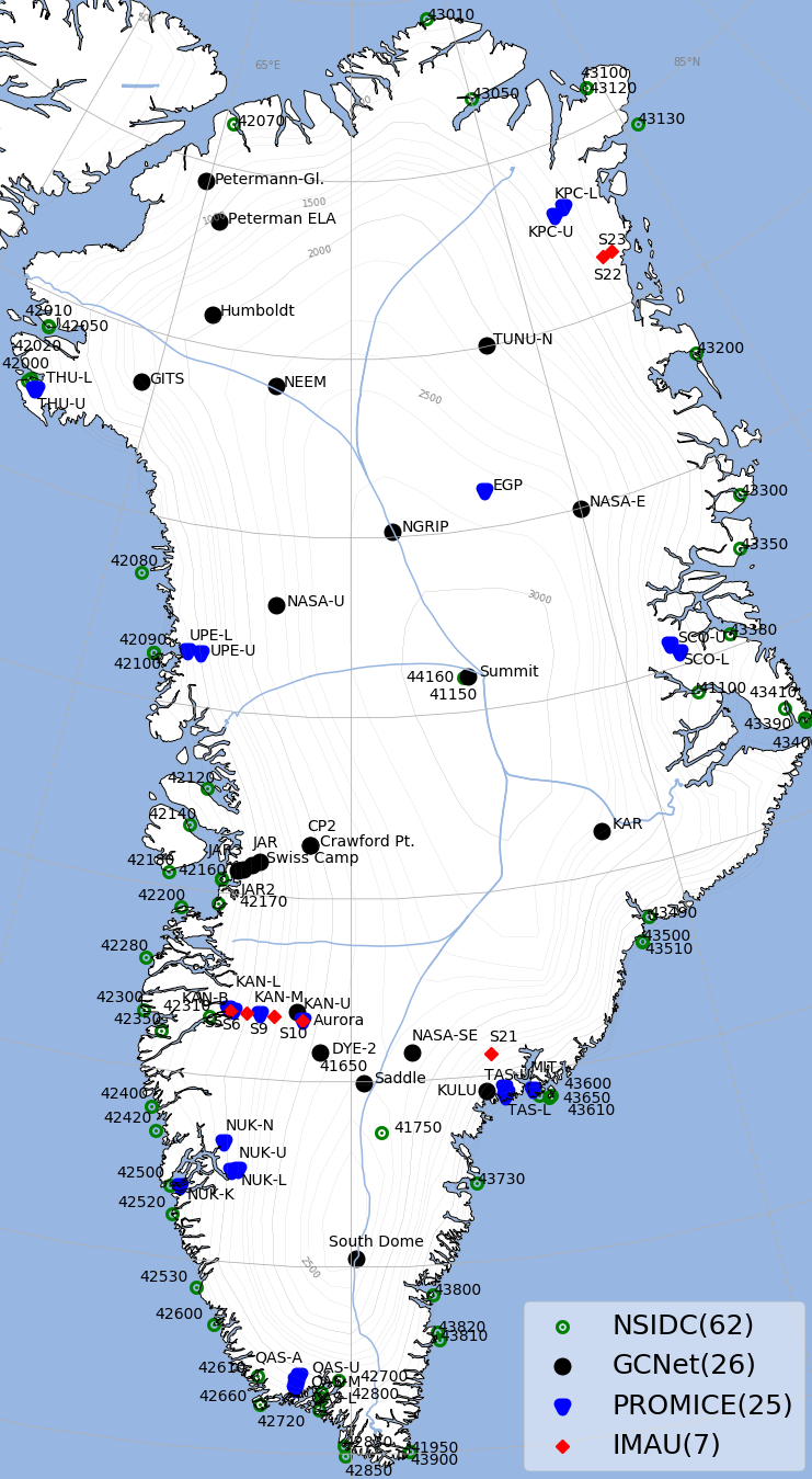
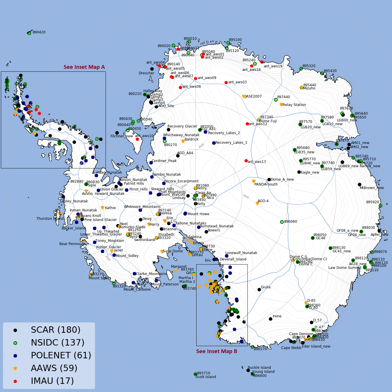
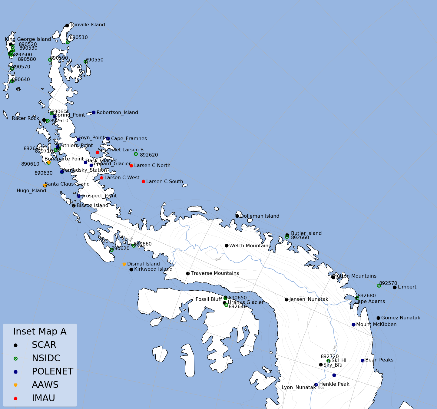
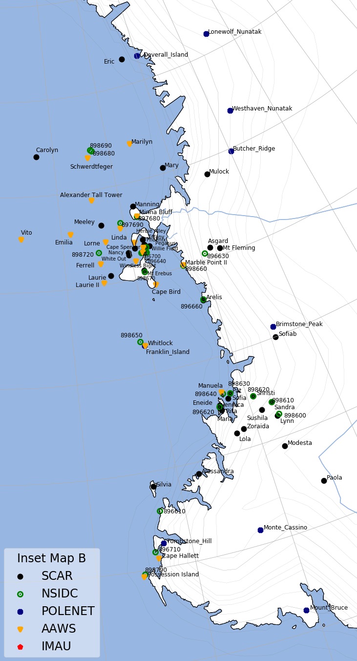
Supported Networks¶

The current version of JAWS can translate L2 ASCII data from the following AWS networks to netCDF format:

AAWS(Antarctic Automatic Weather Stations): They focus on observational Antarctic meteorological research, providing real-time and archived meteorological data and observations.
GCNet(Greenland Climate Network): They collect climate information on Greenland’s ice sheet.
IMAU(Institute for Marine and Atmospheric Research): They have deployed several AWS on glaciers, ice caps and ice sheets, since 1994. These AWS are deployed on different glaciers around the world, in different climate regimes.
POLENET(The Polar Earth Observing Network): It is a global network dedicated to observing the polar regions in a changing world.
PROMICE(Programme for Monitoring of the Greenland Ice Sheet): The aim of PROMICE is to quantify the mass loss from surface melting and iceberg calving through a combination of observation and modelling. Data on the surface climate and melting is collected from a comprehensive network of AWS spanning all regions of the Greenland Ice Sheet margin.
SCAR(Scientific Committee on Antarctic Research): It is an inter-disciplinary committee of the International Science Council (ISC), and was created in 1958. SCAR is charged with initiating, developing and coordinating high quality international scientific research in the Antarctic region.

Note: If your network is not in the above list and you would like it to be supported by JAWS, please open an issue on Github or contact Charlie Zender at zender@uci.edu

Total number of stations handled by JAWS: 378

Total number of station-years of data handled by JAWS: 3600

Download AWS Data¶

We have permission to host only 1-day sample data for each network, which can be downloaded from this webpage. There is one file for each network on the webpage. The file name is prefixed by network name. To save a file, right click on the file name and select “Save link as”.

Important Note:

For PROMICE, input file name must contain station name. 
e.g. 'PROMICE_KAN-B.txt' or 'KAN-B.txt' or 'Kangerlussuaq-B_abc.txt', etc.

For IMAU, input file name must start with network type(i.e. 'ant' or 'grl'), 
followed by a underscore and then station number. 
e.g. 'ant_aws01.txt' or 'ant_aws15_123.txt' or 'grl_aws21abc.txt', etc.

The complete data for each network can be downloaded or requested from following links:

AAWS: http://amrc.ssec.wisc.edu/aws/api/form.html

GCNet: http://cires1.colorado.edu/steffen/gcnet/order/admin/station.php

IMAU: https://www.uu.nl/en/research/imau/contact

POLENET: Data can be obtained via anonymous FTP to ftp.bas.ac.uk in src/SCAR_EGOMA/POLENET_AWS directory.

PROMICE: https://promice.org/PromiceDataPortal/api/download/f24019f7-d586-4465-8181-d4965421e6eb/v03/hourly/csv

SCAR: Data can be obtained via anonymous FTP to ftp.bas.ac.uk in src/SCAR_EGOMA/AWS directory.

Example¶

JAWS is a command-line tool. Linux/Unix users can run JAWS from terminal and Windows users from Anaconda Prompt.

The only required argument that a user has to provide is the input file path. The following minimalist command converts the input ASCII file to netCDF format (using default options):

$ jaws PROMICE_EGP_20160503.txt

By default, the output file will be stored within the current working directory with same name as of input file (e.g. PROMICE_EGP_20160503.txt will be converted to PROMICE_EGP_20160503.nc).

The user can optionally give their own output path/filename using -o option as following:

$ jaws -o ~/Desktop/PROMICE_EGP_20160503.nc PROMICE_EGP_20160503.txt

where the first argument i.e. after -o is the user-defined path to output file and the last argument is path to input file.

All options are explained in detail in the Arguments section.

Important Note:

For PROMICE, input file name must contain station name. 
e.g. 'PROMICE_KAN-B.txt' or 'KAN-B.txt' or 'Kangerlussuaq-B_abc.txt', etc.

For IMAU, input file name must start with network type(i.e. 'ant' or 'grl'), 
followed by a underscore and then station number. 
e.g. 'ant_aws01.txt' or 'ant_aws15_123.txt' or 'grl_aws21abc.txt', etc.

Arguments¶

Positional Arguments¶

input: Path to raw L2 data file for converting to netCDF (or use -i option).
output: Path to save output netCDF file (or use -o option).

Note: input is first positional argument and it is required, whereas output is second (or last) positional argument and it is optional. See examples below to understand more about it.

Case 1: User provides only input (e.g. ‘ABC.txt’).

Usage:

$ jaws ABC.txt

This will convert ‘ABC.txt’ to netCDF format with same name as input file i.e. ‘ABC.nc’.

Case 2: User provides both input (e.g. ‘ABC.txt’) and output file name (e.g. ‘XYZ.nc’).

Usage:

$ jaws ABC.txt XYZ.nc

This will convert ‘ABC.txt’ to ‘XYZ.nc’.

Optional Arguments¶

-i, --fl_in, --input: Path to raw L2 data file for converting to netCDF (or use first positional argument).

Usage:
```
$ jaws -i ABC.txt
```
or
```
$ jaws --fl_in ABC.txt
```
or
```
$ jaws --input ABC.txt
```
-o, --fl_out, --output: Path to save output netCDF file (or use last positional argument).

Usage:
```
$ jaws -i ABC.txt -o XYZ.nc
```
or
```
$ jaws -o XYZ.nc -i ABC.txt
```
-r, --vrs, --version, --revision: JAWS current version and last modified date.

Usage:
```
$ jaws --version America/Los_Angeles ABC.txt
```
-c, --cel, --celsius --centigrade: By default, all temperature variables will be in Kelvin (K) in output file (SI units). Use this option if you want them in Celsius (°C) in output netCDF file. If during analysis step, you find that units are Kelvin and you want the plots in Celsius, first convert the raw file to netCDF using this option and then do the analysis.

Usage:
```
$ jaws --celsius ABC.txt
```
--mb, --hPa, --millibar: By default, all pressure variables will be in Pascal (Pa) in output file (SI units). Use this option if you want them in hPa/millibar in output netCDF file. If during analysis step, you find that units are Pa and you want the plots in hPa, first convert the raw file to netCDF using this option and then do the analysis.

Usage:
```
$ jaws --hPa ABC.txt
```
--rigb: Calculate adjusted downwelling shortwave flux, tilt_angle and tilt_direction. This option is only for stations that archive radiometric data.

Usage:
```
$ jaws --rigb ABC.txt
```
--merra: Select MERRA dataset for thermodynamic profiles in RIGB calculations. It has to be used in conjunction with rigb option.

Usage:
```
$ jaws --rigb --merra ABC.txt
```
-f, --fll_val_flt, --fillvalue_float: Override default float _FillValue.

Usage:
```
$ jaws --fll_val_flt 999.99 America/Los_Angeles ABC.txt
```
-s, --stn_nm, --station_name: Override default station name.

Usage:
```
$ jaws -s AA ABC.txt
```
-t, --tz, --timezone: Change the timezone, default is UTC. A list of all the timezones can be found here.

Usage:
```
$ jaws --timezone America/Los_Angeles ABC.txt
```
-3, --format3, --3, --fl_fmt=classic: Output file in netCDF3 CLASSIC (32-bit offset) storage format.

Usage:
```
$ jaws -3 ABC.txt
```
-4, --format4, --4, --netcdf4: Output file in netCDF4 (HDF5) storage format. This is default.

Usage:
```
$ jaws --format4 ABC.txt
```
-5, --format5, --5, --fl_fmt=64bit_data: Output file in netCDF3 64-bit data (i.e., CDF5, PnetCDF) storage format.

Usage:
```
$ jaws --fl_fmt=64bit_data ABC.txt
```
-6, --format6, --6, --64: Output file in netCDF3 64-bit offset storage format.

Usage:
```
$ jaws --6 ABC.txt
```
-7, --format7, --7, --fl_fmt=netcdf4_classic: Output file in netCDF4 CLASSIC format (3+4=7).

Usage:
```
$ jaws -7 ABC.txt
```
-L, --dfl_lvl, --dfl, --deflate: Lempel-Ziv deflation/compression (lvl=0..9) for netCDF4 output.

Usage:
```
$ jaws --dfl_lvl 2 America/Los_Angeles ABC.txt
```
--flx, --gradient_fluxes: This method is only for GCNet stations. Calculate gradient fluxes i.e. Sensible and Latent Heat Flux based on Steffen & DeMaria (1996). This method is very sensitive to input data quality.

Usage:
```
$ jaws --flx ABC.txt
```
--no_drv_tm, --no_derive_times: By default extra time variables (month, day and hour) are derived for further analysis. Use this option to not derive them.

Usage:
```
$ jaws --no_drv_tm ABC.txt
```
-D, --dbg_lvl, --debug_level: Debug-level ranging from 1 to 9. It prints what steps are occurring during conversion.

Usage:
```
$ jaws -D 5 ABC.txt
```
-a, --anl, --analysis: Plot type e.g.- diurnal, monthly, annual, seasonal.

Usage:
```
$ jaws -a XYZ.nc
```
-v, --var, --variable: Variable you want to analyze.

Usage:
```
$ jaws -a -v temperature ABC.txt
```
-y, --anl_yr, --analysis_year: Year you want to select for analysis.

Usage:
```
$ jaws -a -v temperature -y 2012 ABC.txt
```
-m, --anl_mth, --analysis_month: Month you want to select for analysis.

Usage:
```
$ jaws -a -v temperature -y 2012 -m 5 ABC.txt
```

RIGB Adjustment¶

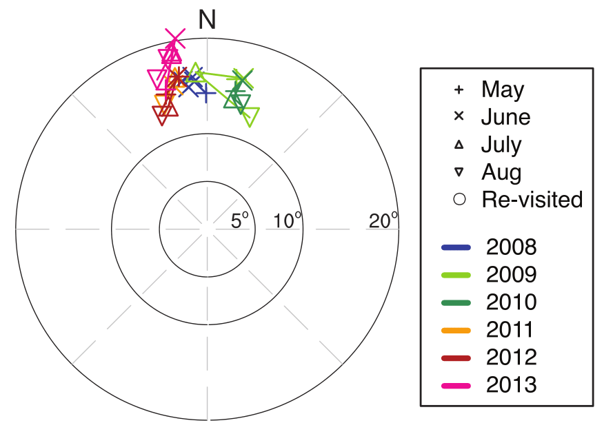
RIGB (Retrospective, Iterative, Geometry-Based) is a method that corrects tilt angle and direction for AWS with solar radiometry. Unattended AWS are subject to tilt, especially when anchored in snow and ice. This tilt can alter the AWS-retrieved albedo from a the expected “smiley face” diurnal profile to almost a frown.

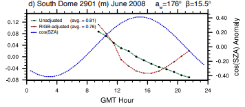
The tilt angle at South Dome station was β ≈ 15◦ in 2008, enough to bias retrieved albedo by 0.05–0.10.

The RIGB tilt-correction algorithm advanced the state-of-the-art in removing surface shortwave biases from AWS. It reduces solar biases by 11Wm−2 averaged over Greenland from May–Sept (Wang et al., 2016), enough to melt 0.24m snow water equivalent.

To run RIGB, user needs to specify “–rigb” option as below:

$ jaws ~/Downloads/gcnet_summit_20120817.txt --rigb

Note: Active internet connection is needed when running RIGB, as RRTM and CERES files will be downloaded for calculations, they will be deleted however upon completion.

RIGB uses climlab’s radiative transfer model to simulate clear-sky radiation.

RIGB relies on three external datasets:

AIRS: for thermodynamic profiles (2002-present)
MERRA: for thermodynamic profiles (1995-present)
CERES: for cloud fractions

AIRS is the default dataset used for thermodynamic profiles in JAWS but AIRS data is available only since 2002. So, users working on pre-2002 datasets, please choose MERRA as following:

$ jaws ~/Downloads/gcnet_summit_20120817.txt --rigb --merra

It is to be noted here that user needs to use ‘–merra’ option in conjunction with ‘–rigb’.

Analysis¶

Currently, the input file for analysis should be in netCDF format. So, first the raw ASCII files should be converted to netCDF using previous steps. We are working to make it accept ASCII files as input.

In the following examples we have used GCNet station at Summit, if you are using a separate network, you need to change the variable name accordingly.

JAWS has the ability to analyze the data in multiple ways such as:

Diurnal¶

JAWS can be used to plot the monthly diurnal cycle to see hourly changes for any variable throughout the month. The user needs to provide the input file path, variable name (on which analysis needs to be done) and analysis type (i.e. diurnal, monthly, annual or seasonal). The argument for analysis is -a, --anl or --analysis and variable name is -v, --var or --variable.

We will take two examples here:

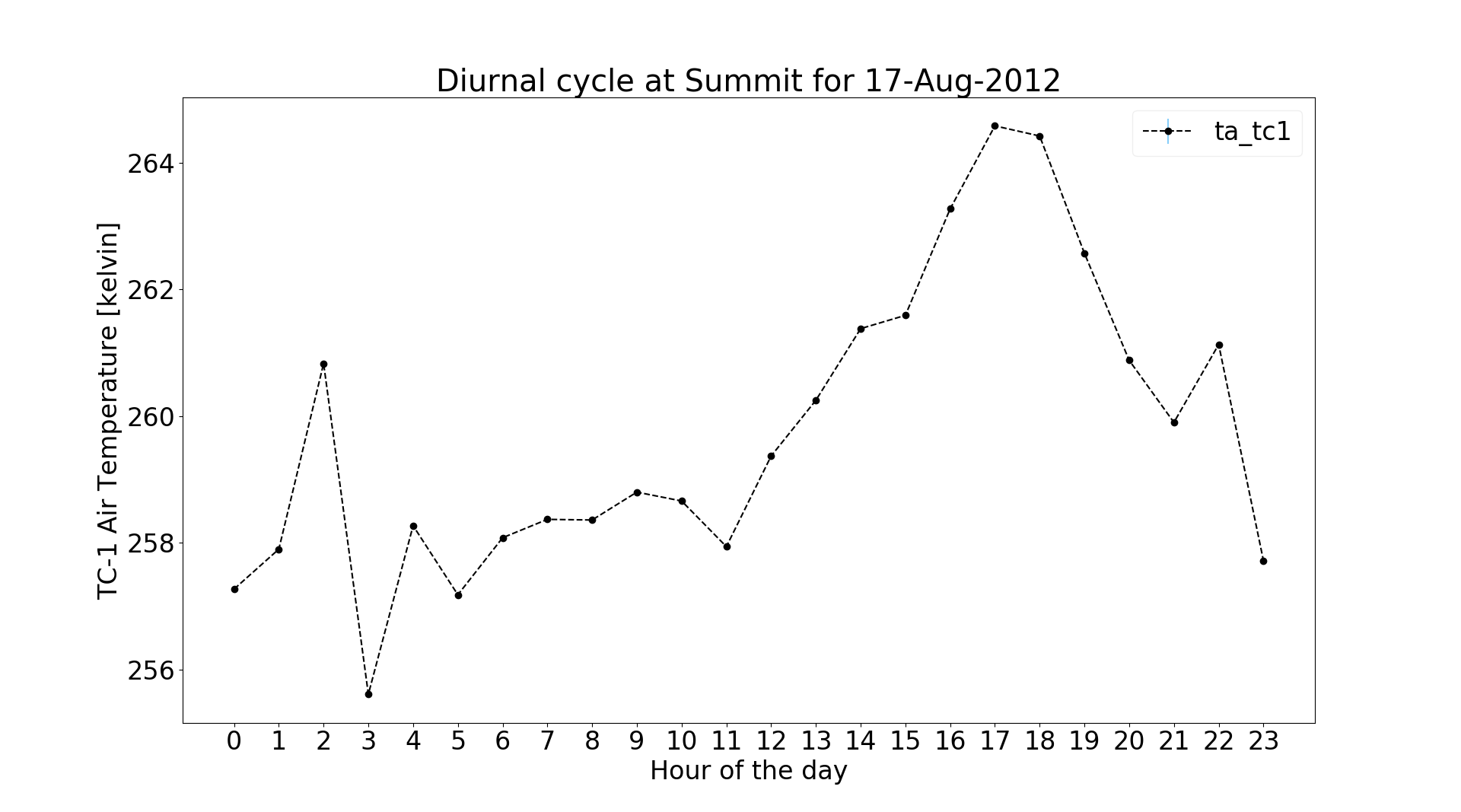
Case 1: The input file contains only 1-day data. We will consider the file converted previously i.e. GCNet_Summit_20120817.nc. By default, the temperature variables will be in Kelvin (K) units in converted netCDF file. If you would like them in Celsius (°C), please use -c, --cel, --celsius --centigrade option when converting the raw file to netCDF. Please note that --analysis option will only use units that are in netCDF file and units can’t be changed during this step.

Use the following command to see how temperature varies throughout the day:
```
$ jaws -a diurnal -v ta_tc1 GCNet_Summit_20120817.nc
```
Case 2: We will be using multi-year data from GCNet-Summit. We don’t have permission to host this data.

Since, there are many years and months in this file, we need to provide for which year and month we want to do the analysis. The argument for year is -y, --anl_yr or --analysis_year and month is -m, --anl_mth or --analysis_month.

If the input file contains data for only single year, then the user doesn’t need to provide the ‘-y’ argument. Similar is the case for ‘-m’ (month) argument.

We will do the analysis for May-2002 at GCNet_Summit:
```
$ jaws -a diurnal -v ta_tc1 -y 2002 -m 5 gcnet_summit.nc
```
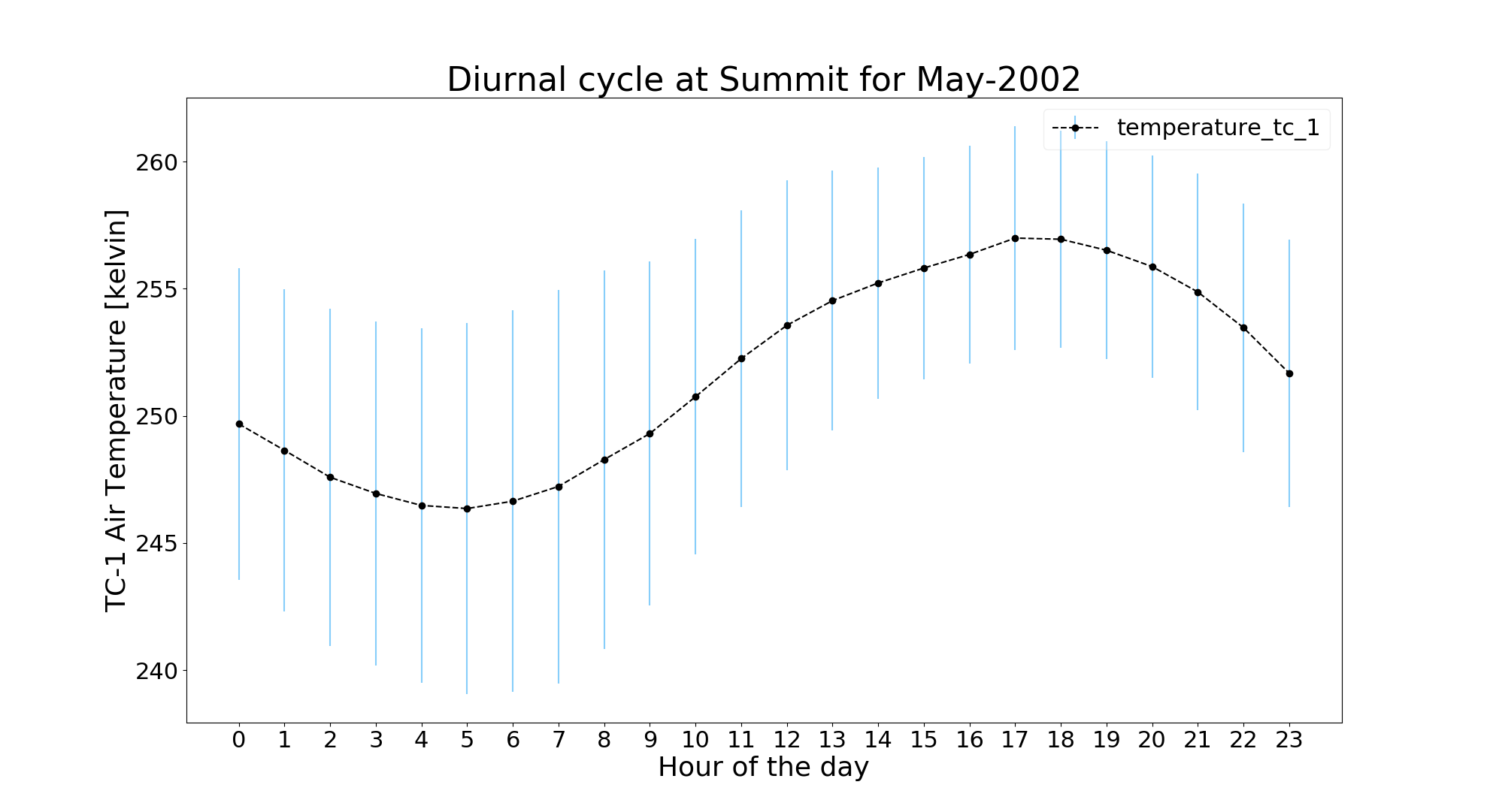
The blue error bar shows standard deviation for that hour across the month.

Important: This same file from Case 2 will be used for the next three analysis because we need at least the monthly, yearly and 
multi-yearly data.

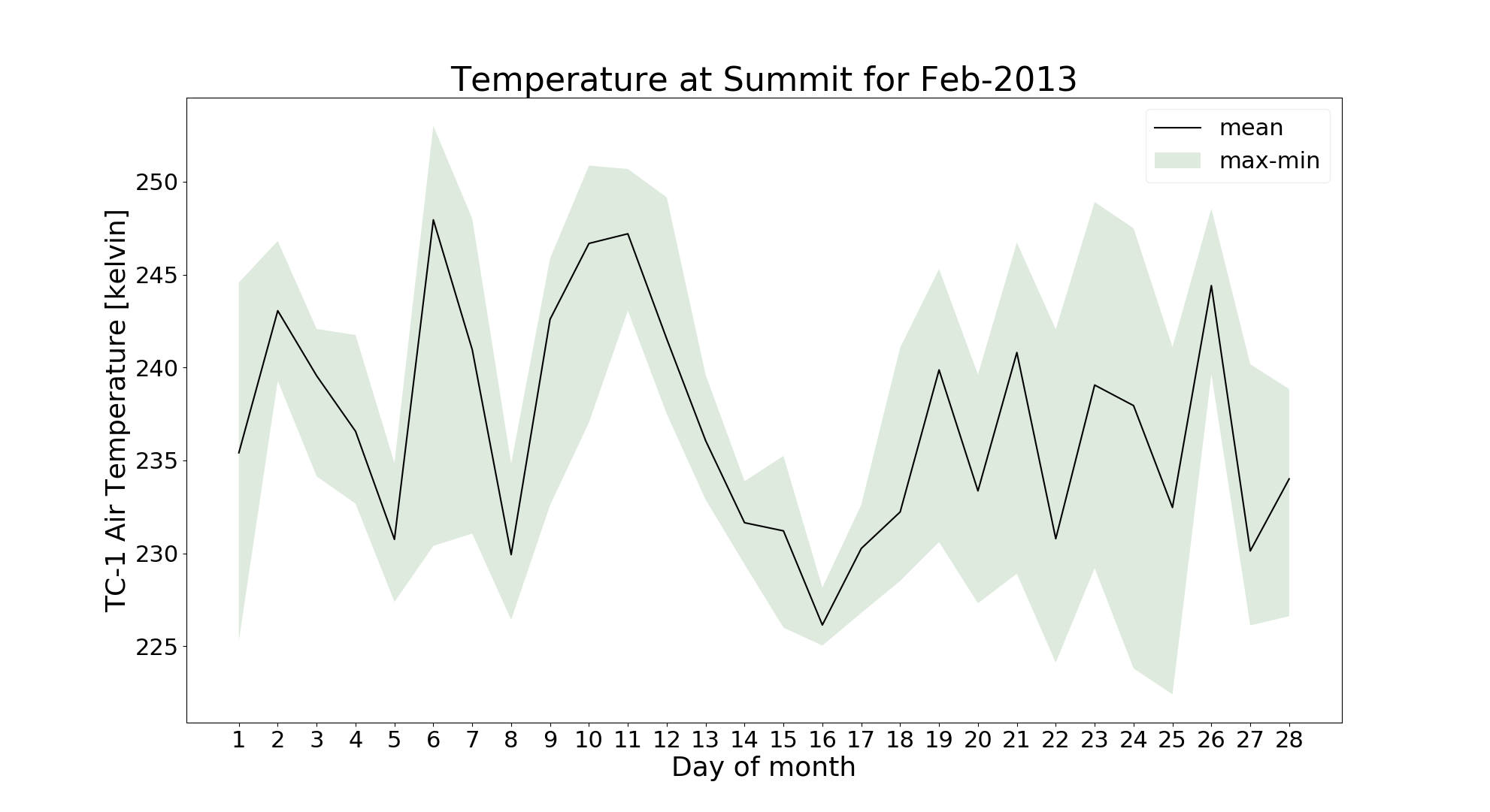
Monthly¶

In this analysis, we can analyze avg, max and min values for each day of a month for any variable

This time we will do it for temperature from a different sensor for Feb-2013 as following:

$ jaws --anl monthly --var ta_cs1 --anl_yr 2013 --anl_mth 2 gcnet_summit.nc

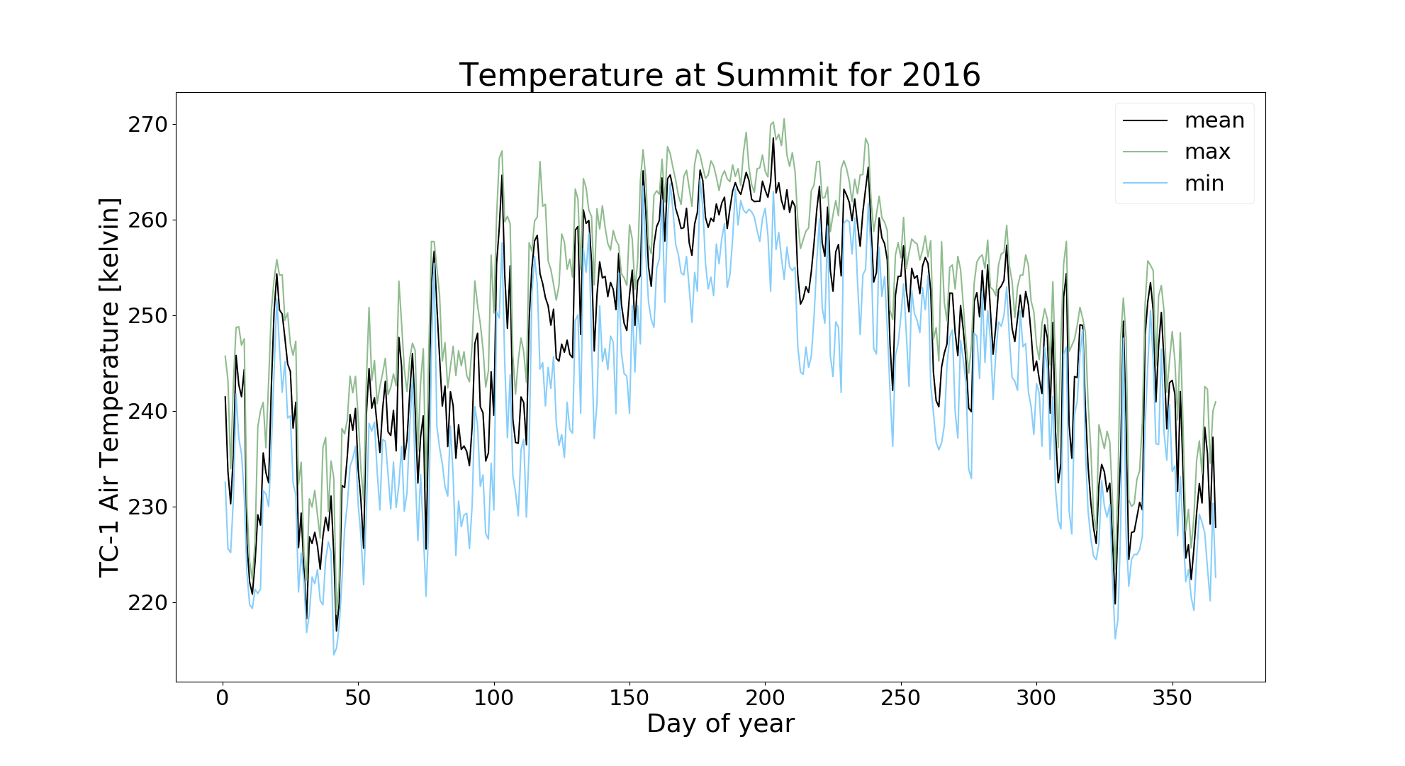
Annual¶

To plot an annual cycle with daily mean, max and min:

$ jaws --analysis annual --variable ta_tc1 --analysis_year 2016 gcnet_summit.nc

Note: Since this is an annual plot, the user shouldn’t provide the ‘-m’ argument

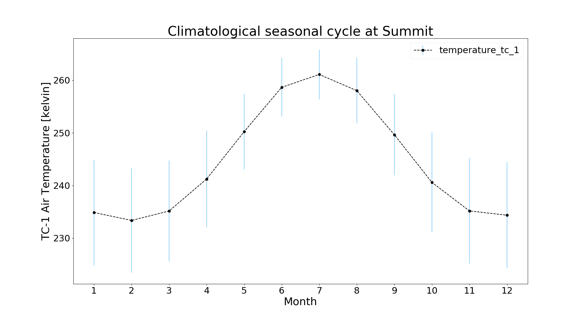
Seasonal¶

Climatological seasonal cycle showing variation for each month through multiple years:

$ jaws -a seasonal -v ta_tc1 gcnet_summit.nc

Note: Since this is a seasonal plot, the user shouldn’t provide both ‘-y’, ‘-m’ argument.

API¶

Adding new variables to an existing network¶

Each network has a list of variables (from raw file) that are known to JAWS at:

jaws/resources/{network_name}/columns.txt

where ‘network_name’ is the name of newtork lke ‘gcnet’, ‘promice’, etc.

If you want to modify JAWS and add new variables to a network, you need to modify following 3 files i.e.

jaws/resources/{network_name}/columns.txt

jaws/resources/{network_name}/ds.json

jaws/resources/{network_name}/encoding.json

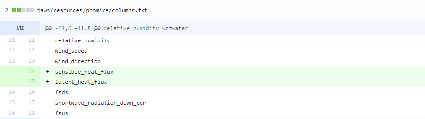
In this example, we will add two new variables (‘Sensible Heat Flux’ and ‘Latent Heat Flux’) to PROMICE.

Step 1: Add variable names to columns.txt of that network in same order as they are in raw file. In our example raw file, ‘sensible_heat_flux’ comes after ‘wind_direction’ and is followed by ‘latent_heat_flux’. So, we will add new variables like this:

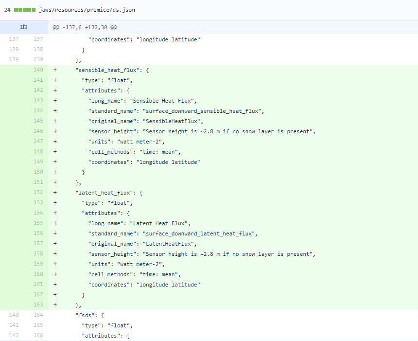
Step 2: Next, we will populate attributes information for the newly added variables in ds.json as following:

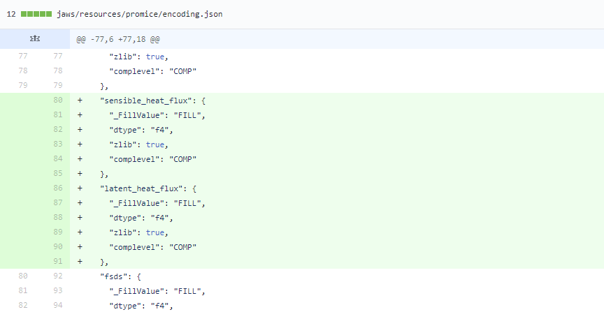
Step 3: Then, we will add the encoding information in encoding.json as below:

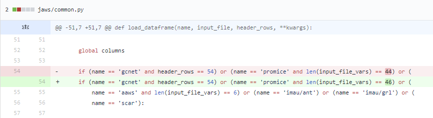
Step 4: The final step is only for AAWS, GCNet and PROMICE networks. You will need to update the count of variables in jaws/common.py. Since we have added two variable, so we will update the len(input_file_vars) from 44 to 46 as following:

If you have trouble following the above or have any questions, please open up an issue on Github

Add new network¶

If your network is not in the list here and you would like it to be supported by JAWS, please open an issue on Github or contact Charlie Zender at zender@uci.edu

Acronyms¶

AAWS: Antarctic Automatic Weather Stations

AIRS: Aeromatic Information Retrieval System (Database)

AWS: Automatic Weather Station

CERES: Cloud and the Earth’s Radiant Energy System

CF: Climate and Forecast Conventions and Metadata

GCNet: Greenland Climate Network

IMAU: Institute for Marine and Atmospheric Research

JAWS: Justified Automated Weather Station

MERRA: Modern-Era Retrospective analysis for Research and Applications

POLENET: The Polar Earth Observing Network

PROMICE: Programme for Monitoring of the Greenland Ice Sheet

RIGB: Retrospective Iterative Geometry-Based

SCAR: Scientific Committee on Antarctic Research

Citing JAWS¶

If JAWS played an important role in your research, then please add us to your reference list using one of the options below.

BibTeX entry¶

Example BibTeX entry::

  @software{jaws,
    author = {Zender, Charlie and Wang, Wenshan and Saini, Ajay },
    organization = {University of California, Irvine},
    title = {JAWS: An Extensible Toolkit to Harmonize and Analyze Polar Automatic Weather Station Datasets, Manuscript in Preparation for Geosci. Model Dev..},
    year = {2017 - 2019},
    version = {1.0},
    url = {https://github.com/jaws/jaws},
    address = {Irvine, California}
  }

AMS Journal Style¶

Example Citation::

  Zender, C. S., Wang, W., Saini A. K., 2019:
      JAWS 1.0: An Extensible Toolkit to Harmonize and Analyze Polar Automatic Weather Station Datasets, Manuscript in Preparation for Geosci. Model Dev..
      [Available online at https://github.com/jaws/jaws]

Github¶

Here is the link to JAWS Github page.

References¶

[Wang 2016] Wang, W., Zender, C. S., van As, D., Smeets, P. C. J. P., & van den Broeke, M. R. (2016). A Retrospective, Iterative, Geometry-Based (RIGB) tilt-correction method for radiation observed by automatic weather stations on snow-covered surfaces: application to Greenland. The Cryosphere, 10(2), 727–741. doi: http://doi.org/10.5194/tc-10-727-2016

[Hobbs1977] Hobbs, P. V., and J. M. Wallace, 1977: Atmospheric Science: An Introductory Survey. Academic Press, 350 pp.

[Salby1996] Salby, M. L., 1996: Fundamentals of Atmospheric Physics. Academic Press, 627 pp.

License¶

Licensed under the Apache License, Version 2.0 (the “License”); you may not use this file except in compliance with the License. You may obtain a copy of the License at http://www.apache.org/licenses/LICENSE-2.0

Unless required by applicable law or agreed to in writing, software distributed under the License is distributed on an “AS IS” BASIS, WITHOUT WARRANTIES OR CONDITIONS OF ANY KIND, either express or implied. See the License for the specific language governing permissions and limitations under the License.