bioLEC - Landscape elevational connectivity¶

Understanding how biodiversity formed and evolved is a key challenge in evolutionary and ecological biology [Newbold2016]. Despite a theoretical consensus on how best to measure biodiversity from a biological perspective (_i.e._ number of species, length of all branches on the tree of life of a species, and differences in allele and genotype frequencies within species) standardised and cost-effective methods for assessing it on a broad range of scales are lacking [Chiarucci2011]. Estimates of some of theses landscape abiotic properties are already available through standard software such as ArcGIS or QGIS and in more specific mountainous landscape focussed packages such as LSD Topo Tools or pyBadlands.

In 2016, a new metric called the Landscape Elevational Connectivity (LEC) was proposed to estimate biodiversity in mountainous landscape [Bertuzzo2016]. It efficiently measures the landscape resistance to migration and is able to account for up to 70% of biodiversity predicted by meta-community models [Bertuzzo2016].

bioLEC is a Python package designed to quickly calculate for any mountainous landscape surface and species niche width its associated LEC index. From an elevational fitness perspective, all migratory paths on a flat landscape are equal. This is not the case on a complex landscape where migration can only occur along a network of corridors providing species with their elevational requirements. Hence, predicting how species will disperse across a landscape requires a model of migration that takes into account the physical properties of the landscape, the species fitness range, as well as evolving environmental conditions.

Note

LEC quantifies the closeness of a site to all others with similar elevation. It measures how easily a species living in a given patch can spread and colonise other patches. It is assumed to be elevation-dependent and the metric depends on how often a species adapted to a given elevation needs to travel outside its optimal elevation range when moving from its patch to any other in the landscape. bioLEC package can be used in serial or parallel to evaluate biodiversity patterns of a given landscape. It is an efficient and easy-to-use tool to quickly assess the capacity of landscape to support biodiversity and to predict species dispersal across mountainous landscapes.

Contents¶

What is the LEC?¶

LEC quantifies the closeness of a site to all others with similar elevation. For a given landscape, LEC is primarily dependent on elevation range and on species niche width. It quantifies the closeness of any point in the landscape to all others at similar elevation.

It has been shown that LEC captures well the \(\alpha\)-diversity variations observed in mountainous landscape [Lomolino2008] and simulated by full meta-community models [Bertuzzo2016] as shown in the figure below.

Important

It suggests that geomorphic features are a first-order control on biodiversity and that LEC metric can be used to quickly assess species richness distribution in complex landscapes.

Cost function¶

Considering a 2D lattice made of N squared cells, LEC for cell i (\({LEC}_i\)) is given by

\[{LEC}_i = \sum_{j=1}^N C_{ji}\]

where \(C_{ji}\) quantifies the closeness between sites j and i with respect to elevational connectivity. \(C_{ji}\) measures the cost for a given species adapted to cell j to spread and colonise cell i. This cost is a function of elevation and evaluates how often species adapted to the elevation of cell j have to travel outside their optimal species niche width (\(\sigma\)) to reach cell i (as shown in the figure below).

Following Bertuzzo et al. [Bertuzzo2016], \(C_{ji}\) is expressed as:

\[-\ln C_{ji} = \frac{1}{2\sigma^2} \min_{p \in \{j\rightarrow i\}} \sum_{r=2}^L (z_{k_r}-z_j)^2\]

where \(p=[k_1,k_2, ...,k_L]\) (with \(k_1=j\) and \(k_L=i\)) are the cells comprised in the path p from j to i.

In the figure above, we illustrate the approach implemented in bioLEC to compute the closeness measure (\(C_{ji}\)) used to quantify LEC based on a topography grid (adapted from [Bertuzzo2016]). Two paths from site j to i (inset) are proposed with their elevation profiles. Associated costs are computed following the equation above (\(\sum_{r=2}^L (z_{k_r}-z_j)^2\)).

Hint

Despite a longer length, the cost associated to the red path is smaller than that of the blue one as it passes across sites with similar elevations to \(z_j\).

Dijkstra’s algorithm ¶

The estimation of \(C_{ji}\) requires computation of all the possible paths p from j to i and is defined as the maximum closeness value along these paths and this is solved for each cell j using Dijkstra’s algorithm [Dijkstra1959] with diagonal connectivity between cells.

For each cell j, the algorithm builds a Dijkstra tree that branches the given cell with all the cells defining the simulated region. Edge weights are set equal to the square of the difference between the considered vertex elevation (\(z_{k_r}\)) and \(z_j\). The least-cost distance between j and i is then calculated as the minimum sum of edge weights obtained from the cells along the shortest-path (see top figure).

Here, the closeness is measured as a least-cost distances that optimises the costs associated to the edge weights of the traversed cells as well as the travelled Euclidean distance. As the least-cost distances incorporate landscape costs to movement, the approach allows for closeness differentiation between cells that might be seen as equally near if landscape costs were not accounted for.

In bioLEC we rely on scikit-image to compute the least cost distances [Etherington2017]. scikit-image package is primarily intended to process image [vanderWalt2014] but is designed to work with NumPy arrays making it compatible with other Python packages (e.g. most other geospatial Python packages) and really simple to use with digital elevation datasets.

While scikit-image uses slightly different terminology, talking about minimum cost paths rather than least-cost paths, the approach is identical to those commonly implemented in GIS software and applies Dijkstra’s algorithm with diagonal connectivity between cells [Etherington2016].

Parallelisation¶

Dijkstra’s algorithm is a graph search algorithm that solves single-source shortest path for a graph with non-negative weights. Such an algorithm can be quite long to solve especially in bioLEC as it needs to be used to compute the least-cost paths for every points on the surface.

Here we do not perform a parallelisation of the Dijkstra’s algorithm but instead we adopt a simpler strategy where the Dijkstra trees for all paths are balanced and distributed over multiple processors using message passing interface (MPI). The approach consists in splitting the computational domain row-wise as shown in the above figure. Least-cost paths are then computed for the points belonging to each sub-domain using the Dijkstra’s algorithm over the entire region.

Note

Using this approach, LEC computation is significantly reduced and scales really well with increasing CPUs.

[Bertuzzo2016]

(1, 2, 3) E. Bertuzzo, F. Carrara, L. Mari, F. Altermatt, I. Rodriguez-Iturbe & A. Rinaldo - Geomorphic controls on species richness. PNAS, 113(7) 1737-1742, DOI: 10.1073/pnas.1518922113, 2016.

[Dijkstra1959]

E.W. Dijkstra - A note on two problems in connexion with graphs. Numer. Math. 1, 269-271, DOI: 10.1007/BF01386390, 1959.

[Etherington2016]

T.R. Etherington - Least-cost modelling and landscape ecology: concepts, applications, and opportunities. Current Landscape Ecology Reports 1:40-53, DOI: 10.1007/s40823-016-0006-9, 2016.

[Etherington2017]

T.R. Etherington - Least-cost modelling with Python using scikit-image, Blog, 2017.

[Lomolino2008]

M.V. Lomolino - Elevation gradients of species-density: historical and prospective views. Glob. Ecol. Biogeogr. 10, 3-13, DOI: 10.1046/j.1466-822x.2001.00229.x, 2008.

[vanderWalt2014]

S. van der Walt, J.L. Schönberger, J. Nunez-Iglesias, F. Boulogne, J.D. Warner, N. Yager, E. Gouillart & T. Yu - Scikit Image Contributors - scikit-image: image processing in Python, PeerJ 2:e453, 2014.

Installation¶

bioLEC is a pure Python package and can be installed via pip as well as Docker.

Dependencies¶

You will need Python 2.7 or 3.5+ and the following packages are required: numpy, scipy, pandas, mpi4py, scikit-image, pyevtk.

Note

The mpi4py module has to be installed as a wrapper around an existing installation of MPI. The easiest way to install it is to use anaconda, which will install a compatible version of MPI and configure mpi4py to use it: conda install -c conda-forge mpi4py

The complete list of Dependencies is available in the src/requirements.txt file and looks like:

numpy>=1.15
six>=1.11.0
setuptools>=38.4.0
mpi4py>=3.0.0
pandas>=0.24
scipy>=1.2
scikit-image>=0.15
pyevtk>=1.1.1
matplotlib>=3.0
rasterio>=1.0.23

Optionally, lavavu is needed to support interactive visualisation in Jupyter environment (as shown in the notebook examples available from binder).

Installing using pip¶

You can install bioLEC package using the latest stable release available via pip!

pip install bioLEC

If you need to install it for different python versions:

$ python2 -m pip install bioLEC
$ python3 -m pip install bioLEC

To install the development version: Clone the repository using

git clone https://github.com/Geodels/bioLEC.git

Navigate into the bioLEC directory and run

$ cd src/
$ pip install -r requirements.txt
$ pip install .

Installing using Docker¶

Another straightforward installation which does not depend on specific compilers relies on docker virtualisation system.

To install the docker image and test it is working:

$ docker pull geodels/biolec:latest
$ docker run --rm geodels/biolec:latest help

On Linux, to build the dockerfile locally, we provide a script. First ensure you have checked out the source code from github and then run the script in the Docker directory. If you modify the dockerfile and want to push the image to make it publicly available, it will need to be retagged to upload somewhere other than the GEodels repository.

$ git checkout https://github.com/Geodels/bioLEC.git
$ cd bioLEC
$ source Docker/build-dockerfile.sh

Note

For non-Linux platforms, the use of Docker Desktop for Mac or Docker Desktop for Windows is recommended. The docker container to look for is named geodels/biolec!

Testing installation¶

A test is provided to check the correct installation of the bioLEC package.If you’ve cloned the source into a directory bioLEC, you may verify it as follows:

Navigate the the directory src/tests and run the tests.

$ python2 testInstall.py
$ python3 testInstall.py

You will need to have all dependencies installed.

The following result indicates success.

$ Test bioLEC installation:: [####################] 100.0% DONE
$ All tests were successful...

Quick start guide¶

I/O Options¶

The most simple code lines to use bioLEC package is summarised below

import bioLEC as bLEC

biodiv = bLEC.landscapeConnectivity(filename='pathtofile.csv')
biodiv.computeLEC()

biodiv.writeLEC('result')
biodiv.viewResult(imName='plot.png')

Input¶

The entry point is the function landscapeConnectivity() (see API landscapeConnectivity) that requires the elevation field as it main input. There are 3 ways to import the elevation dataset :

as a CSV file (argument: filename) containing 3 columns for X, Y and Z respectively with no header and ordered along the X axis first (as illustrated in the top figure) and shown below:

\[\begin{split}\begin{smallmatrix} x_0 & y_0 & z_{0,0} \\ x_1 & y_0 & z_{1,0} \\ \vdots & \vdots & \vdots \\ x_m & y_0 & z_{m,0} \\ x_0 & y_1 & z_{0,1} \\ \vdots & \vdots & \vdots \\ x_m & y_n & z_{m,n} \\ \end{smallmatrix}\end{split}\]
as a 3D numpy array (argument: XYZ) containing the X, Y and Z coordinates here again ordered along the X axis first (as above)
or as a 2D numpy array (argument: Z) containing the elevation matrix (example provided below), in this case the dx argument is also required

\[\begin{split}\begin{smallmatrix} z_{0,0} & z_{1,0} & \cdots & z_{m-1,0} & z_{m,0} \\ \vdots & \vdots & \vdots & \vdots & \vdots \\ z_{0,k} & z_{1,k} & \cdots & z_{m-1,k} & z_{m,k} \\ \vdots & \vdots & \vdots & \vdots & \vdots \\ z_{0,n} & z_{1,n} & \cdots & z_{m-1,n} & z_{m,n} \\ \end{smallmatrix}\end{split}\]

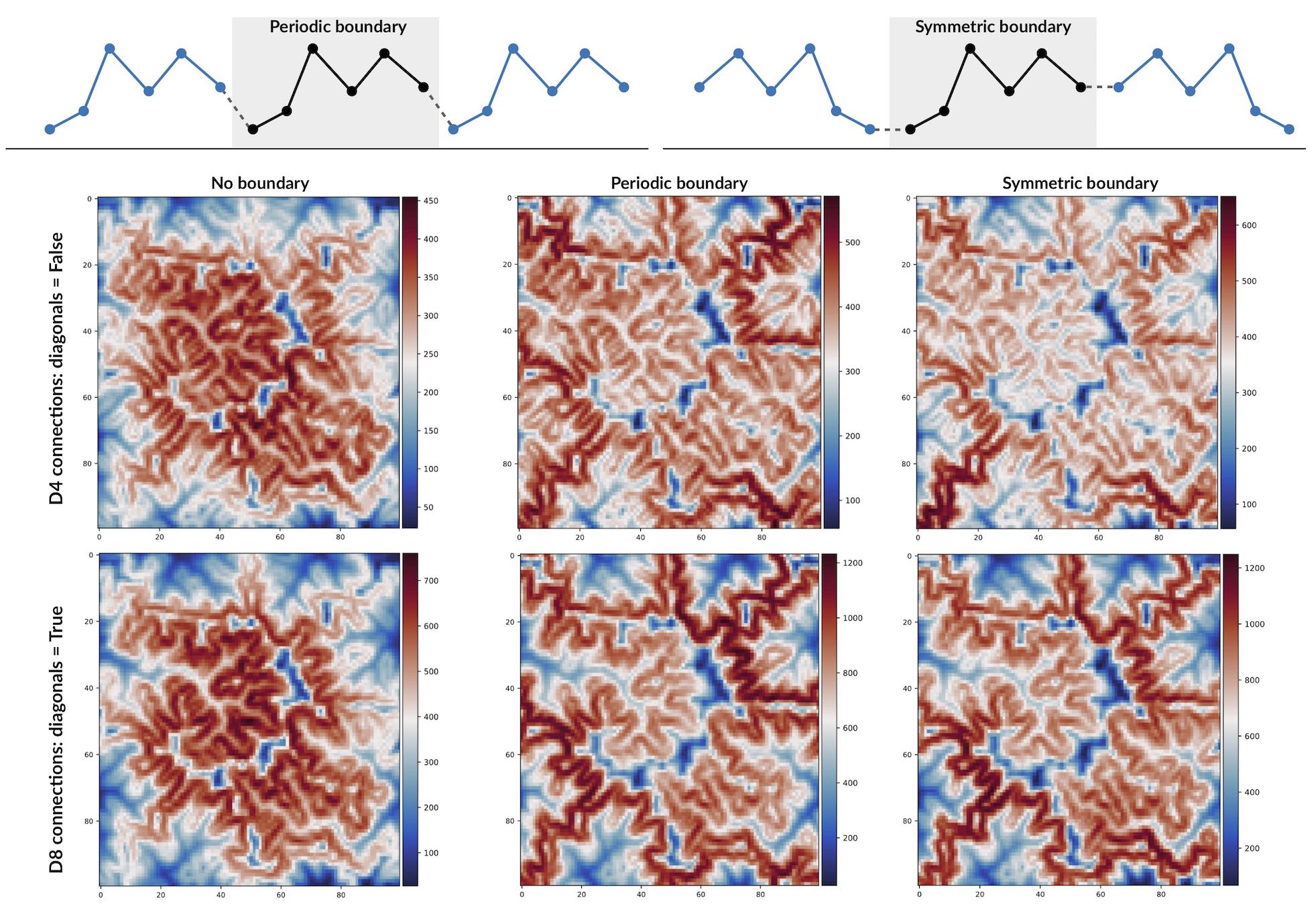
In addition to the elevation field, the user could specify the boundary conditions used to compute the LEC. Two options are available: periodic or symmetric boundaries. The way these two boundaries are implemented in bioLEC is illustrated in the figure below as well as the impact on the LEC calculation.

Finally the LEC solution requires the declaration of the species niche width defined by the variable sigma in the following equation (look in the What is LEC? section for more information):

\[-\ln C_{ji} = \frac{1}{2\sigma^2} \min_{p \in \{j\rightarrow i\}} \sum_{r=2}^L (z_{k_r}-z_j)^2\]

The above figure from [Bertuzzo16] shows the habitat maps as a function of elevation for a real fluvial landscape when considering the fitness of three different species as a function of elevation. The fitness maps of the three species are shown on the bottom panels. In bioLEC two options are possible:

either the user specifies a species niche width percentage based on elevation extent with the parameter sigmap
or a species niche fixed width values with the declaration of the parameter sigmav

Outputs¶

import bioLEC as bLEC

biodiv = bLEC.landscapeConnectivity(filename='pathtofile.csv')
biodiv.computeLEC()

biodiv.writeLEC('result')
biodiv.viewResult(imName='plot.png')

Once the computeLEC() function (see API compute LEC) has been ran, the result are then available in different forms.

From the writeLEC function (see API write LEC), the user can first save the dataset in CSV and VTK formats containing the X,Y,Z coordinates as well as the computed LEC and normalised LEC (_nLEC_).

Then several figures can be created showing maps of elevation and LEC values as well as graphs of LEC and elevation frequency as a function of site elevation (such as the figure presented below). In some functions, one can plot the average and error bars of LEC within elevational bands.

Available plotting functions are provided below:

viewResult
viewElevFrequency
viewLECFrequency
viewLECZbar
viewLECZFrequency

For a complete list of available options, users need to go to the API documentation.

Running examples¶

There are different ways of using the bioLEC package. If you used a local install with pip, you can download the Jupyter Notebooks provided in the Github repository…

$ git clone https://github.com/Geodels/bioLEC.git

Binder & Docker¶

The series of Jupyter Notebooks can also be ran with Binder that opens those notebooks in an executable environment, making the package immediately reproducible without having to perform any installation.

This is by far the most simple method to test and try this package, just launch the demonstration at bioLEC-live (mybinder.org)!

Another straightforward installation that again does not depend on specific compilers relies on the docker virtualisation system. Simply look for the following Docker container geodels/biolec.

Note

For non-Linux platforms, the use of Docker Desktop for Mac or Docker Desktop for Windows is recommended.

HPC & Terminal¶

The tool can be used to compute the LEC for any landscape file as long as the data is available from a CSV file containing 3D coordinates (X,Y,Z) with no header and space delimiter.

Attention

Notebooks environment will not be the best option for large landscape models and we will recommend the use of the python script: runLEC.py in HPC environment.

In this case, the code will be ran from a terminal like this:

$ mpirun -np XX python runLEC.py -i 'xyzfile.csv' -o 'result'

where XX represents the number of processors to use.

The python script runLEC.py is provided in the same folder as the Jupyter notebooks and is defined by:

import argparse
from mpi4py import MPI
import bioLEC as LEC

comm = MPI.COMM_WORLD
size = comm.Get_size()
rank = comm.Get_rank()

# Parsing command line arguments
parser = argparse.ArgumentParser(description='This is a simple entry to run bioLEC package from python.',add_help=True)

# Required
parser.add_argument('-i','--input', help='Input file name (csv file)',required=True)
parser.add_argument('-o','--output',help='Output file name without extension', required=True)

# Optional
parser.add_argument('-p','--periodic',help='True/false option for periodic boundary conditions', required=False, action="store_true", default=False)
parser.add_argument('-s','--symmetric',help='True/false option for symmetric boundary conditions', required=False, action="store_true", default=False)
parser.add_argument('-w','--width',help='Float option for species niche width percentage', required=False, action="store_true", default=0.1)
parser.add_argument('-f','--fix',help='Float option for species niche width fix values', required=False, action="store_true", default=None)
parser.add_argument('-c','--diagonals',help='True/false option for computing the path based on the diagonal moves as well as the axial ones eg. D4/D8 connectivity', required=False, action="store_true", default=True)
parser.add_argument('-n','--nout',help='Number for output frequency during run', required=False, action="store_true", default=500)
parser.add_argument('-d','--delimiter',help='String for elevation grid csv delimiter', required=False,action="store_true",default=' ')
parser.add_argument('-l','--level',help='Float for sea level position', required=False,action="store_true",default=-1.e6)
parser.add_argument('-v','--verbose',help='True/false option for verbose', required=False,action="store_true",default=False)

args = parser.parse_args()
if args.verbose and rank == 0:
  print("Required arguments: ")
  print("   + Input file: {}".format(args.input))
  print("   + Output file without extension: {}".format(args.output))
  print("\nOptional arguments: ")
  print("   + Periodic boundary conditions for the elevation grid: {}".format(args.periodic))
  print("   + Symmetric boundary conditions for the elevation grid: {}".format(args.symmetric))
  print("   + Species niche width percentage based on elevation extent: {}".format(args.width))
  print("   + Species niche width based on elevation extent: {}".format(args.fix))
  print("   + Computes the path based on the diagonal moves as well as the axial ones: {}".format(args.diagonals))
  print("   + Elevation grid csv delimiter: {}".format(args.delimiter))
  print("   + Sea level position: {}".format(args.level))
  print("   + Number for output frequency: {}\n".format(args.nout))

biodiv = LEC.landscapeConnectivity(filename=args.input,periodic=args.periodic,symmetric=args.symmetric,
                                    sigmap=args.width,sigmav=args.fix,diagonals=args.diagonals,
                                    delimiter=args.delimiter,sl=args.level)

biodiv.computeLEC(args.nout)

biodiv.writeLEC(args.output)

if rank == 0:
    biodiv.viewResult(imName=args.output+'.png')
    biodiv.viewElevFrequency(input=args.output,imName=args.output+'_zfreq.png')
    biodiv.viewLECZFrequency(input=args.output,imName=args.output+'_leczfreq.png')
    biodiv.viewLECFrequency(input=args.output,imName=args.output+'_lecfreq.png')
    biodiv.viewLECZbar(input=args.output,imName=args.output+'_lecbar.png')

[Bertuzzo16]

E. Bertuzzo, F. Carrara, L. Mari, F. Altermatt, I. Rodriguez-Iturbe & A. Rinaldo - Geomorphic controls on species richness. PNAS, 113(7) 1737-1742, DOI: 10.1073/pnas.1518922113, 2016.

Collaborations¶

How to contribute¶

We welcome all kinds of contributions! Please get in touch if you would like to help out.

Important

Everything from code to notebooks to examples and documentation are all equally valuable so please don’t feel you can’t contribute.

To contribute please fork the project make your changes and submit a pull request. We will do our best to work through any issues with you and get your code merged into the main branch.

If you found a bug, have questions, or are just having trouble with bioLEC, you can:

join the bioLEC User Group on Slack by sending an email request to: tristan.salles@sydney.edu.au
open an issue in our issue-tracker and we’ll try to help resolve the concern.

Where to find support¶

Please feel free to submit new issues to the issue-log to request new features, document new bugs, or ask questions.

License¶

This program is free software: you can redistribute it and/or modify it under the terms of the GNU Lesser General Public License as published by the Free Software Foundation, either version 3 of the License, or (at your option) any later version.

API documentation¶

This section of the documentation details the auto-generated API from Read the Docs.

class bioLEC.LEC.landscapeConnectivity(filename=None, XYZ=None, Z=None, dx=None, periodic=False, symmetric=False, sigmap=0.1, sigmav=None, diagonals=True, delimiter=' ', sl=-1000000.0, test=False)[source]¶

Bases: object

Landscape elevational connectivity (LEC) quantifies the closeness of a site to all others with similar elevation. Such closeness is computed over a graph whose edges represent connections among sites and whose weights are proportional to the cost of spreading through patches at different elevation.

Method:: E. Bertuzzo et al., 2016: Geomorphic controls on elevational gradients of species richness - PNAS doi

Parameters:

filename (str) – CSV file name containing regularly spaced elevation grid [default: None]
XYZ (3D Numpy Array) – 3D coordinates array of shape (nn,3) where nn is the number of points [default: None]
Z (2D Numpy Array) – Elevation array of shape (nx,ny) where nx and ny are the number of points along the X and Y axis [default: None]
dx (float) – grid spacing in metre when the Z argument defined above is used [default: None]
periodic (bool) – applied periodic boundary to the elevation grid see explanation [default: False]
symmetric (bool) – applied symmetric boundary to the elevation grid see explanation [default: False]
sigmap (float) – species niche width percentage based on elevation extent [default: 0.1]
sigmav (float) – species niche fixed width values [default: None]
diagonals (bool) – computes the path based on the diagonal moves as well as the axial ones eg. D4/D8 connectivity [default: True]
delimiter (str) – elevation grid csv delimiter [default: ‘ ‘]
sl (float) – sea level position used to remove marine points from the LEC calculation [default: -1.e6]

Caution

There are 3 ways to import the elevation dataset in bioLEC:

either as a CSV file (argument: filename) containing 3 columns for X, Y and Z respectively with no header and ordered along the X axis first

or as a 3D numpy array (argument: XYZ) containing the X, Y and Z coordinates here again ordered along the X axis first

or as a 2D numpy array (argument: Z) containing the elevation matrix, in this case the dx argument is also required

Note

It is worth noting that the boundary conditions are either symmetric or periodic. Although LEC simply depends on the elevation field and on the niche width, LEC predicts well the alpha-diversity simulated by full metacommunity models.

computeLEC(fout=500)[source]¶

This function computes the minimum path for all nodes in a given surface and measure of the closeness of each node to other at similar elevation range.

It then provide the landscape elevational connectivity array from computed measure of closeness calculation.

Parameters:	fout (int) – output frequency [default: 500]

computeMinPath(r, c)[source]¶

Internal function to compute the minimum path between a specific node and all other ones.

Parameters:	c (int) – row indice of the consider point r (int) – column indice of a consider point
Returns:	minimum-cost path for the specified node.
Return type:	mincost

Note

This function relies on scikit-image (image processing in python) and finds distance-weighted minimum cost paths through an n-d costs array.

splitRowWise()[source]¶

Rowwise block partitioning used to perform LEC computation in parallel.

Returns:	number of nodes to consider on each partition startID (1D array int): starting index for each partition endID (1D array int): ending index for each partition
Return type:	disps (1D array int)

Note

From the number of processors (np) available split the array into equal number row wise.

viewElevFrequency(input=None, imName=None, nbins=80, size=(6, 6), fsize=11, dpi=200)[source]¶

This function plots and saves in a figure the distribution of elevation.

Parameters:	input (str) – CSV file name containing the dataset imName (str) – (string) image name with extension nbins (int) – number of bins for the histogram (default: 80) size – size of the image [default: (6,6)] fsize (int) – title font size [default: 11] dpi (int) – resolution of the saved image [default: 200]

Warning

The filename needs to be provided without extension.

viewLECFrequency(input=None, imName=None, size=(6, 6), fsize=11, dpi=200)[source]¶

This function plots and saves in a figure the distribution of LEC with elevation.

Parameters:	input (str) – CSV file name containing the dataset imName (str) – (string) image name with extension size – size of the image [default: (6,6)] fsize (int) – title font size [default: 11] dpi (int) – resolution of the saved image [default: 200]

Warning

The filename needs to be provided without extension.

viewLECZFrequency(input=None, imName=None, size=(6, 6), fsize=11, dpi=200)[source]¶

This function plots and saves in a figure the distribution of LEC and elevation with elevation.

Parameters:	input (str) – CSV file name containing the dataset imName (str) – (string) image name with extension size – size of the image [default: (6,6)] fsize (int) – title font size [default: 11] dpi (int) – resolution of the saved image [default: 200]

Warning

The filename needs to be provided without extension.

viewLECZbar(input=None, imName=None, nbins=40, size=(6, 6), fsize=11, dpi=200)[source]¶

This function plots and saves in a figure the distribution of LEC and elevation with elevation as well as the standard deviation for LEC values for each bins.

Parameters:	input (str) – CSV file name containing the dataset imName (str) – (string) image name with extension nbins (int) – number of bins for the histogram (default: 40) size – size of the image [default: (6,6)] fsize (int) – title font size [default: 11] dpi (int) – resolution of the saved image [default: 200]

Warning

The filename needs to be provided without extension.

viewResult(imName=None, size=(9, 5), fsize=11, cmap1=<matplotlib.colors.LinearSegmentedColormap object>, cmap2=<matplotlib.colors.LinearSegmentedColormap object>, dpi=200)[source]¶

This function plots and saves in a figure the result of the LEC computation.

Parameters:	imName (str) – (string) image name with extension size – size of the image [default: (9,5)] fsize (int) – title font size [default: 11] cmap1 – color map for elevation grid [default: plt.cm.summer_r] cmap2 – color map for LEC grid [default: cmap2=plt.cm.coolwarm] dpi (int) – resolution of the saved image [default: 200]

writeLEC(filename='LECout')[source]¶

This function writes the computed landscape elevational connectivity array in a CSV file and create a VTK visualisation file (.vts).

Parameters:	filename (str) – output file name without format extension.

Warning

The filename needs to be provided without extension.

Indices and tables¶

[Newbold2016]

T. Newbold, et al. - Has land use pushed terrestrial biodiversity beyond the planetary boundary? A global assessment. Science, 353(6296) 288-291, `DOI: 10.1126/science.aaf2201`_, 2016.

[Chiarucci2011]

A. Chiarucci, G. Bacaro, & S. Scheiner - Old and new challenges in using species diversity for assessing biodiversity. Phil. Trans. R. Soc. B Biol Sci., 366(1576) 2426-2437, `DOI: 10.1098/rstb.2011.0065`_,2011.

[Bertuzzo2016]

(1, 2) E. Bertuzzo, F. Carrara, L. Mari, F. Altermatt, I. Rodriguez-Iturbe & A. Rinaldo - Geomorphic controls on species richness. PNAS, 113(7) 1737-1742, `DOI: 10.1073/pnas.1518922113`_, 2016.

bioLEC - Landscape elevational connectivity¶

Contents¶

What is the LEC?¶

Cost function¶

Dijkstra’s algorithm¶

Parallelisation¶

Installation¶

Dependencies¶

Installing using pip¶

Installing using Docker¶

Testing installation¶

Quick start guide¶

I/O Options¶

Input¶

Outputs¶

Running examples¶

Binder & Docker¶

HPC & Terminal¶

Collaborations¶

How to contribute¶

Where to find support¶

License¶

API documentation¶

Indices and tables¶

Dijkstra’s algorithm ¶