Welcome to the documentation of the MULTIPLY platform!
Introduction
Multiply EU-Horizon 2020 project
“MULTIscale SENTINEL land surface information retrieval Platform”
With the start of the SENTINEL era, an unprecedented amount of Earth Observation (EO) data will become available. Currently there is no consistent but extendible and adaptable framework to integrate observations from different sensors in order to obtain the best possible estimate of the land surface state. MULTIPLY proposes a solution to this challenge.
The project will develop an efficient, fully generic and fully traceable platform that uses state-of-the-art physical radiative transfer models, within advanced data assimilation (DA) concepts, to consistently acquire, interpret and produce a continuous stream of high spatial and temporal resolution estimates of land surface parameters, fully characterized. These inferences on the state of the land surface will be the result from the coherent joint interpretation of the observations from the different Sentinels, as well as other 3rd party missions (e.g. ProbaV, Landsat, MODIS).

radiative transfer models
The framework allows users to exchange components as plug-ins according to their needs and builds on the EO-LDAS concepts, which have shown the feasibility of producing estimates of the land surface parameters by combining different sets of observations through the use of radiative transfer models. The data retrieval platform will operate in an environment with advanced visualisation tools.
Users will be engaged throughout the process and trained. Moreover, user demonstrator projects include applications to crop monitoring & modelling, forestry, biodiversity and nature management. Another user demonstrator project involves providing satellite operators with an opportunity to cross-calibrate their data to the science-grade Sentinel standards.
The project will run from 1st January 2016 till 31 December 2019.
Components
In this section, the various components that form the MULTIPLY platform are explained in detail.
MULTIPLY Data Access
This is the help for the MULTIPLY Data Access Component (DAC). The DAC forms part of the MULTIPLY platform, which is a platform for the retrieval of bio-physical land parameters (such as fAPAR or LAI) on user-defined spatial and temporal grids from heterogeneous data sources, in particular from EO data in the microwave domain (Sentinel-1), optical high resolution domain (Sentinel-2), and optical coarse resolution domain (Sentinel-3). The DAC has been designed to work as part of the platform, but can also be used separately to manage and query for data from local and remote sources.
The MULTIPLY Data Access Component serves to access all data that is required by components of the MULTIPLY platform. It can be queried for any supported type of data for a given time range and spatial region and provide URL’s to the locally provided data. In particular, the Data Access Component takes care of downloading data that is not yet available locally.
The Data Access Component relies on the concept of Data Stores: All data is organized in such a data store. Such a store might provide access to locally stored data or encapsulate access to remotely stored data. Users may register new data stores and, if they find that the provided implementations are not sufficient, implement their own data store realizations.
This help is organized into the following sections.
Basic Concepts
Basically, the Data Access Component administrates several Data Stores. A Data Store is a unit that provides access to data of a certain type. It consists of a FileSystem and a MetaInfoProvider. The FileSystem accesses the actual data, the MetaInfoProvider has information on the available data.

This separation has been undertaken so that queries can be performed quickly on the MetaInfoProvider without having to browse through the FileSystem which might be costly. Queries on the availability of data for a given data type, spatial region, and in a certain time range will be addressed to the MetaInfoProvider. Such information will be retrieved in the form of a DataSetMetaInfo object. This is a simple data storage object which provides information about the data type, spatial coverage, start time and end time of a dataset.
The File System will be addressed when actual URL’s are requested. Such a request might result in costly operations, such as downloads.
Some of the Data Stores access data that is stored remotely. To make it accessible to the other components of the MULTIPLY platform it needs to be downloaded and added to a local data store. These remote data stores are “wrapped” by a local data store, so the result is a store that has a remote File System, a local File System, a remote Meta Info Provider and a local Meta Info Provider.

If a query is made for data, the Data Store will search first in the local, then in the remote Meta Info Provider. Results from the remote Meta Info Provider that are already contained in the local Meta Info Provider will not be considered. When then the data is actually requested, it is either simply retrieved from the local File System or, if it is provided on the remote File System, downloaded from there into a temporary directory. It is then put into the local File System and the local Meta Info Provider is updated with the information about the newly added data.
The following forms of FileSystems and MetaInfoProviders exist:
File Systems:
LocalFileSystem: Provides access to locally stored data. Applicable to any data type, this is the default for local meta info provision.
HttpFileSystem: A locally wrapped file system that retrieves data via http. Applicable to any data type.
AWSS2FileSystem: A locally wrapped file system that retrieves S2 data in the AWS format from the Amazon Web Services. This File System requires that users are registered at the AWS.
LpDaacFileSystem: A locally wrapped file system that retrieves MODIS MCD43A1.006 data from the Land Processes Distributed Active Archive Center. This File System requires that users have an Earthdata Login.
VrtFileSystem: A locally wrapped file system that downloads data sets of a given type, a certain spatial region and no temporal information. It combines these data sets into a single global .vrt-file which references the downloaded data sets. This is useful for ,e.g., having elevation data.
Meta Info Providers:
JsonMetaInfoProvider: A local meta info provider that stores relevant information (spatial coverage, start time, end time, data type) about a data set in a JSON file. Applicable to any data type, this is the default for local meta information provision.
HttpMetaInfoProvider: A locally wrapped meta info provider that provides meta information about data sets that can be retrieved via http. Applicable for any data type.
AwsS2MetaInfoProvider: A locally wrapped meta info provider that provides meta information about S2 data in the AWS format from the Amazon Web Services. This information can be retrieved without having an AWS account.
LpDaacMetaInfoProvider: A locally wrapped meta info provider that provides meta information about MODIS MCD43A1.006 data from the Land Processes Distributed Active Archive Center. This File System requires that users have an Earthdata Login.
VrtMetaInfoProvider: A locally wrapped meta info provider that provides meta information about a single global .vrt-file that encapsulates access to data sets from a given data type.
Installation
Requirements
The MULTIPLY Data Access Component has been developed against Python 3.6. It cannot be guaranteed to work with previous Python versions, so we suggest using 3.6 or higher. The DAC will attempt downloading data from remote sources. We therefore recommend to run it on a computer which has a lot of storage (solid state disks are recommended) and also a good internet connection.
Installing from source
To install the Data Access Component, you need to clone the latest version of the MULTIPLY code from GitHub and step into the checked out directory:
cd data-access
To install the MULTIPLY Data Access into an existing Python environment just for the current user, use:
python setup.py install –user
To install the MULTIPLY Data Access for development and for the current user, use
python setup.py develop –user
Configuration
There are a few configuration options you can make to use the DAC. These options will be available after you use the DAC for the first time. To use it, type in a python console:
$ from multiply_data_access import DataAccessComponent
$ dac = DataAccessComponent()
When you execute this for the first time, in your home directory a folder .multiply is created,
in which you will find a file called data_stores.yml ,
which we will refer to as the data stores file in the following.
This file contains the data stores to which the DAC has access.
In the beginning, it will consist of several default entries for data stores
which are required for accessing remote data
(For an explanation of the concepts of a FileSystem and a MetaInfoProvider go to function).
These entries have settings that look like the following:
- DataStore:
FileSystem:
parameters:
path: /path/to/user_home/.multiply/aws_s2/
pattern: /dt/yy/mm/dd/
temp_dir: /path/to/user_home/.multiply/aws_s2/temp/
type: AwsS2FileSystem
Id: aws_s2
MetaInfoProvider:
parameters:
path_to_json_file: /path/to/user_home/.multiply/aws_s2/aws_s2_store.json
type: AwsS2MetaInfoProvider
Consider especially the parameters path and pattern of the FileSystem.
These parameters determine where downloaded data will be saved.
path determines the root path, pattern determines a pattern for adding an additional relative graph.
dt stands here for the data type, yy for the year, mm for the month, and dd for the day of the month.
So, if you download S2 L1C data in the AWS format for the 26th of April, 2018,
using the above configuration it would be saved to
/path/to/user_home/.multiply/aws_s2/aws_s2_l1c/2018/4/26/.
Feel free to change these parameters so the data is stored where you want it.
If you point it to a folder that already contains data, make sure it conforms to the pattern so it will be detected.
If you want to add a new data store using your already locally stored data, go to User Guide.
Some of the data stores require authentication. Here we will describe how to set this up the access to Sentinel-2 data from Amazon Web Services (AWS, https://registry.opendata.aws/sentinel-2/ ) and to MODIS data from the Land Processes Distributed Active Archive Center (LP DAAC, https://lpdaac.usgs.gov ) .
Configuring Access to MODIS Data from the LP DAAC
To access the data, you need an Earthdata Login.
If you do not have such a login, click here1_ to register.
.. _here1: https://urs.earthdata.nasa.gov/home
Registration and Data Access are free of charge.
When you have the Login data, open the data stores file and search for the Data Store with the Id MODIS Data.
You will find two entries username and password.
Enter there your Earthdata username and password.
The entry should then look something like this:
- DataStore:
FileSystem:
type: LpDaacFileSystem
parameters:
temp_dir: /path/to/user_home/.multiply/modis/
username: earthdata_login_user_name
password: earthdata_login_password
path: /path/to/data/modis/
pattern: /dt/yy/mm/dd/
Id: MODIS Data
MetaInfoProvider:
type: LpDaacMetaInfoProvider
parameters:
path_to_json_file: /path/to/user_home/.multiply/modis/modis_store.json
Then simply save the file.
Configuring Access to Sentinel-2 Data from Amazon Web Services
First, you can enable it to download Sentinel-2 data from Amazon Web Services.
Please note that unlike the other forms of data access, this one eventually costs money.
The charge is small, though.
(see here2_).
.. _here2: https://forum.sentinel-hub.com/t/changes-of-the-access-rights-to-l1c-bucket-at-aws-public-datasets-requester-pays/172
To enable access, go to https://aws.amazon.com/free/ and sign up for a free account.
You can then log on to the `Amazon Console`__.
__ aws_console_
.. _aws_console: https://console.aws.amazon.com/console/home
From the menu items Services->Security, Identity and Compliance choose ÌAM.
There, under Users, you can add a new user.
Choose a user name and make sure the check box for Programmatic Access is checked.
.. figure:: _static/figures/aws_add_user.png
- scale
50%
- align
center
On the next page you need to set the permissions for the user.
Choose Attach existing policies directly and check the boxes for AmazonEC2FullAccess and AmazonS3FullAccess
(later you may simply choose to copy the permissions from an existing user).
.. figure:: _static/figures/aws_add_user_permissions.png
- scale
50%
- align
center
When everything is correct, you can create the user. On the next site you will be shown the access key id and a secret access key. You can also download both in form of a .csv-file.
Next you will need to install the sentinelhub python package.
Follow the instructions from `this site`__ to do so.
__ sentinelhub_
.. _sentinelhub: https://sentinelhub-py.readthedocs.io/en/latest/install.html
Then proceed to configure sentinelhub using your AWS credentials, following the instructions from `this site`__.
__ sentinelhub_configuration_
.. _sentinelhub_configuration: https://sentinelhub-py.readthedocs.io/en/latest/configure.html
The MULTIPLY Data Access Component will then be able to access this data.
(one can argue that maybe to put this higher up in the structure, but considering that this is only done once, I thought it better to put it lower in the documentation).
User Guide
The MULTIPLY Data Access Component is supposed to be used via its Python API. Therefore, most of this section will deal with the Usage via the Python API. To see how to manually manipulate the data stores file, see Configuration. If you want to register a new data store from data that is saved on local disk, see How to add new Local Data Stores. Finally, if you find that the Data Access Component is missing functionality, you can extend it by Implementing a new File System or Implementing a new Meta Info Provider. When you have these two set up, you can create a new data store by editing the default data stores yaml file.
implementing new file systems
implementing new meta info providers
implementing new data types
Usage via the Python API
This section gives an overview about how the Data Access Component can be used within Python. The only component that is supposed to be used directly is the DataAccessComponent object.
DataAccessComponent
-
class
multiply_data_access.data_access_component.DataAccessComponent[source]¶ The controlling component. The data access component is responsible for communicating with the various data stores and decides which data is used from which data store.
-
can_put(data_type: str) → bool[source]¶ - Parameters
data_type – A data type.
- Returns
True, if data of this type can be added to at least one data store.
-
create_local_data_store(base_dir: Optional[str] = None, meta_info_file: Optional[str] = None, base_pattern: Optional[str] = '/dt/yy/mm/dd/', id: Optional[str] = None, supported_data_types: Optional[str] = None)[source]¶ Adds a a new local data store and saves it permanently. It will consist of a LocalFileSystem and a JsonMetaInfoProvider. :param supported_data_types: A string with the comma-separated names of data types shall be allowed in this data store. If this is None or empty, the data types will be derived from the data sets in the json file. If there are no entries in the json file, it will be guessed from the data in the file system. :param base_dir: The base directory to which the data shall be written. :param meta_info_file: A JSON file that already contains meta information about the data that is present in the folder. If not provided, an empty file will be created and filled with the data that match the base directory and the base pattern. :param base_pattern: A pattern that allows to create an order in the base directory. Available options are ‘dt’ for the data type, ‘yy’ for the year, ‘mm’ for the month, and ‘dd’ for the day, arrangeable in any oder. If no pattern is given, all data will simply be written into the base directory. :param id: An identifier for the Data Store. If there already exists a Data Store with the name, an additional number will be added to the name.
-
get_data_urls(roi: str, start_time: str, end_time: str, data_types: str) → List[str][source]¶ Builds a query from the given parameters and asks all data stores whether they contain data that match the query. If datasets are found, url’s to their positions are returned. :return: a list of url’s to locally stored files that match the conditions given by the query in the parameter.
-
get_data_urls_from_data_set_meta_infos(data_set_meta_infos: List[multiply_data_access.data_access.DataSetMetaInfo]) → List[str][source]¶ Builds a query from the given parameters and asks all data stores whether they contain data that match the query. If datasets are found, url’s to their positions are returned. :return: a list of url’s to locally stored files that match the conditions given by the query in the parameter.
-
get_provided_data_types() → List[str][source]¶ - Returns
A list of all data types that are provided by the Data Access Component.
-
put(path: str, data_store_id: Optional[str] = None) → None[source]¶ Puts data into the data access component. If the id to a data store is provided, the data access component will attempt to put the data into the store. If data cannot be added to that particular store, it will not be attempted to put it into another one. If no store id is provided, the data access component will on its own try to determine an apt data store. A data store is considered apt if it already holds data of the same type. :param path: A path to the data that shall be added to the Data Access Component. :param data_store_id: The id of a data store. Can be None.
-
query(roi: str, start_time: str, end_time: str, data_types: str) → List[multiply_data_access.data_access.DataSetMetaInfo][source]¶ Distributes the query on all registered data stores and returns meta information on all data sets that meet the conditions of the query. :param roi: The region of interest, given in the form of a wkt-string. :param start_time: The start time of the query, given as a string in UTC time format :param end_time: The end time of the query, given as a string in UTC time format :param data_types: A list of data types to be queried for. :return: A list of DataSetMetaInfos that meet the conditions of the query.
-
DataSetMetaInfo
-
class
multiply_data_access.data_access.DataSetMetaInfo(coverage: str, start_time: Optional[str], end_time: Optional[str], data_type: str, identifier: str, referenced_data: Optional[str] = None)[source]¶ A representation of meta information about a data set. To be retrieved from a query on a MetaInfoProvider or DataStore.
-
property
coverage¶ The dataset’s spatial coverage, given as WKT string.
-
property
data_type¶ The type of the dataset.
-
property
end_time¶ The dataset’s end time. Can be none.
-
equals(other: object) → bool[source]¶ Checks whether two data set meta infos are equal. Does not check the identifier or referenced data sets!
-
equals_except_data_type(other: object) → bool[source]¶ Checks whether two data set meta infos are equal, except that they may have the same data type. Does not check the identifier or referenced data sets!
-
property
identifier¶ An identifier so that the data set can be found on the Data Store’s File System.
-
property
referenced_data¶ A list of additional files that are referenced by this data set. Can be none.
-
property
start_time¶ The dataset’s start time. Can be none.
-
property
How to add new Local Data Stores
You can add a new local data store via the Python API like this. This will create a new data store consisting of a LocalFileSystem and a JsonMetaInfoProvider.
All parameters are optional.
The default for the base directory is the .multiply-folder in the user’s home directory.
The base directory will be checked for any pre-existing data.
This data will be registered in the store if it is of any of the supported data types.
If you do not specify the supported data types, the Data Access Component will determine these from the entries in the
JSON metainfo file.
If no metadata file is provided, the data types will be determined from the data in the base directory.
If finally no data can be found there, the data store is not created.
Implementing new Data Stores
If you need to create a completely new data store, you will probably need to implement both a new File System and a new Meta Info Provider (we advise to check whether you can re-use existing File Systems and Meta Info Providers). This section is a guideline on how to do so. It is recommended to consider Basic Concepts first.
Implementing a new File System
The basic decision is whether the file system shall be wrapped by a local file system or not.
The wrapping functionality is provided by the LocallyWrappedFileSystem in locally_wrapped_data_access.py.
Choose this if you want to access remote data but don’t want to bother with how to organize the data on the local disk.
For this, you need to adher to the interfaces FileSystemAccessor and FileSystem defined in data_access.py.
The following lists the methods of the interface that need to be implemented:
-
class
multiply_data_access.data_access.FileSystemAccessor[source]
name: Shall return the name of the file system.
create_from_parameters: Will receive a list of parameters and create a file system by handing these in as the
initialization parameters.
Shall correspond to the dictionary handed out by FileSystem’s get_parameters_as_dict.
-
class
multiply_data_access.data_access.FileSystem[source]¶ An abstraction of a file system on which data sets are physically stored
-
abstract
get(data_set_meta_info: multiply_data_access.data_access.DataSetMetaInfo) → Sequence[<Mock name='mock.FileRef' id='140205175433312'>][source]¶ Retrieves a sequence of ‘FileRef’s.
-
abstract
get_parameters_as_dict() → dict[source]¶ - Returns
The parameters of this file system as dict
-
abstract
put(from_url: str, data_set_meta_info: multiply_data_access.data_access.DataSetMetaInfo) → multiply_data_access.data_access.DataSetMetaInfo[source]¶ Adds a data set to the file system by copying it from the given url to the expected location within the file system. Returns an updated data set meta info.
-
abstract
name: Shall simply return the name of the file system.
This will serve as identifier.
get: From a list of :ref:`ug_02`s, this returns FileRefs to the data that is ready to be accessed, i.e.,
is provided locally.
This part would perform a download if necessary.
get_parameters_as_dict: This will return the parameters that are needed to reconstruct the file system.
The parameters will eventually be written to the data stores file.
Shall correspond to the dictionary handed in by the FileSystemAccessors’s create_from_parameters.
can put: Shall return true when the Data Access Component can add data to the file system.
put: Will copy the data located from the url to the file system and update the data set meta info.
You might throw a User Warning here if you do not support this operation.
You can use the identifier of the data set meta info to later relocate the file on the file system more easily.
remove: Shall remove the file identified by the data set meta info from the file system.
You might throw a User Warning here if you do not support this operation.
scan: Retrieves data set meta infos for all data that is found on the file system.
This expects to find the data that is directly, i.e, locally available.
To later have the file system available in the data access component,
you need to register it in the setup.py of your python package.
The registration should look like this:
- setup(name=’my-multiply-data-access-extension’,
version=1.0, packages=[‘my_multiply_package’], entry_points={
- ‘file_system_plugins’: [
‘my_file_system = my_multiply_package:my_file_system.MyFileSystemAccessor’
],
}, )
A locally wrapped file system requires a FileSystemAccessor that should be defined as above.
The LocallyWrappedFileSystem base class already implements some of the methods,
but puts up other method stubs that need to be implemented.
Note that all these methods are private.
Already implemented methods are:
* get
* get_parameters_as_dict
* can_put
* put
* remove
* scan
So, actually the only method from the FileSystem interface that still needs implementing is name.
-
class
multiply_data_access.locally_wrapped_data_access.LocallyWrappedFileSystem(parameters: dict)[source]¶ -
abstract
_get_from_wrapped(data_set_meta_info: multiply_data_access.data_access.DataSetMetaInfo) → Sequence[<Mock name='mock.FileRef' id='140205175433312'>][source]¶ Retrieves the file ref from the wrapped file system.
-
abstract
_get_wrapped_parameters_as_dict() → dict[source]¶ - Returns
The parameters of this wrapped file system as dict
-
abstract
_init_wrapped_file_system: This method is called right after the creation of the object.
Implement it to initialize the file system with parameters.
Shall correspond to the dictionary handed out by _get_wrapped_parameters_as_dict.
_get_from_wrapped: Like get from the File System: Will retrieve FileRefs to data.
This data has to be provided locally, so any downloading has to be performed here.
_notify_copied_to_local: Informs the File System that the data desidnated by the data set meta info has been put to
the local file system.
You do not have to do anythin here, but in case you have downloaded the data to a temporary directory,
this is a good time to delete it from there.
_get_wrapped_parameters_as_dict: Similar to the FileSystem’s get_parameters_as_dict, this method will return
the required initialization parameters in the form of a dictionary.
Shall correspond to the dictionary handed in to _init_wrapped_file_system.
Implementing a new Meta Info Provider
In many cases when you require your own dedicated File System, you will want to add a Meta Info Provider.
As for the File System, you also have the choice to create a locally wrapped version of it or not.
The wrapping functionality is provided by the LocallyWrappedMetaInfoProvider in locally_wrapped_data_access.py.
Choose this if you want to provide information about remotely stored data and keep it separated from information
about data from this source that has already been downloaded.
To implement a regular Meta Info Provider, you need to create realizations of the interfaces
MetaInfoProviderAccessor and MetaInfoProvider defined in data_access.py.
The MetaInfoProviderAccessor is required by the DataAccessComponent so that MetaInfoProviders can be registered and
created.
The following lists the methods of the MetaInfoProviderAccessor interface that need to be implemented:
-
class
multiply_data_access.data_access.MetaInfoProviderAccessor[source]
name: Shall return the name of the meta info provider.
create_from_parameters: Will receive a list of parameters and create a meta infor provider by handing the
parameters in as the initialization parameters.
Shall correspond to the dictionary handed out by the MetaInfoProvider’s _get_parameters_as_dict.
The methods to be implemented for the MetaInfoProvider are:
-
class
multiply_data_access.data_access.MetaInfoProvider[source]¶ An abstraction of a provider that contains meta information about the files provided by a data store.
-
abstract
_get_parameters_as_dict() → dict[source]¶ - Returns
The parameters of this file system as dict
-
abstract
get_all_data() → Sequence[multiply_data_access.data_access.DataSetMetaInfo][source]¶ Returns all available data set meta infos.
-
abstract
get_provided_data_types() → List[str][source]¶ - Returns
A list of the data types provided by this data store.
-
abstract
provides_data_type(data_type: str) → bool[source]¶ Whether the meta info provider provides access to data of the queried type :param data_type: A string labelling the data :return: True if data of that type can be requested from the meta info provider
-
abstract
query(query_string: str) → List[multiply_data_access.data_access.DataSetMetaInfo][source]¶ Processes a query and retrieves a result. The result will consist of all the data sets that satisfy the query. :return: A list of meta information about data sets that fulfill the query.
-
abstract
name: Shall simply return the name of the meta info provider.
This will serve as identifier.
query: Evaluates a query string and returns a list of data set meta infos about available data that fulfils the
query.
A query string consists of a geometry in the form of a wkt string, a start time in UTC format,
an end time in UTC format, and a comma-separated list of data types.
provides_data_type: True, if the meta info provider is apt for this data.
Returning true here does not necessarilyy mean that data of this type is currently stored.
get_provided_data_types: Returns a list of all data types that this meta info provider supports.
_get_parameters_as_dict: A private method that will return the parameters that are needed to reconstruct
the meta info provider.
The parameters will eventually be written to the data stores file.
Shall correspond to the dictionary handed in by the MetaInfoProviderAccessors’s create_from_parameters.
can_update: Shall return true when entries about data available on the file system can be added to this
meta info provider.
update: Hands in a data set that has been put to the file system.
The meta info provider is expected to store this information and retrieve it when it meets an incoming query.
If this is not implemented, make sure that can_update returns false.
remove: Shall remove the entry associated with the data set meta info from the provider’s registry.
If this is not implemented, make sure that can_update returns false.
get_all_data: Shall return data set meta infos about all available data.
As for the File System, the Meta Info Provider needs to be registered in the setup.py of the python package to
make it available for the data access component.
The registration should look like this:
- setup(name=’my-multiply-data-access-extension’,
version=1.0, packages=[‘my_multiply_package’], entry_points={
- ‘meta_info_provider_plugins’: [
‘my_meta_info_provider = my_multiply_package:my_meta_info_provider.MyMetaInfoProviderAccessor’
],
}, )
A locally wrapped meta info provider is a special type of meta info provider and requires a MetaInfoProviderAccessor
that should be defined as above.
The LocallyWrappedMetaInfoProvider base class already implements some of the methods,
but puts up other method stubs that need to be implemented.
Note that all these methods are private and are never to be called from another class.
Already implemented methods are:
* query
* _get_parameters_as_dict
* can_update
* update
* remove
* get_all_data
So, the only methods from the MetaInfoProvider interface that still needs implementing are name,
provides_data_type, and get_provided_data_types.
-
class
multiply_data_access.locally_wrapped_data_access.LocallyWrappedFileSystem(parameters: dict)[source] -
abstract
_get_wrapped_parameters_as_dict() → dict[source] - Returns
The parameters of this wrapped file system as dict
-
abstract
_init_wrapped_meta_info_provider: This method is called right after the creation of the object.
Implement it to initialize the meta info provider with parameters.
Shall correspond to the dictionary handed out by _get_wrapped_parameters_as_dict.
_query_wrapped_meta_info_provider: Evaluates a query string and returns a list of data set meta infos about
available data that fulfils the query.
A query string consists of a geometry in the form of a wkt string, a start time in UTC format,
an end time in UTC format, and a comma-separated list of data types.
_get_wrapped_parameters_as_dict: Similar to the FileSystem’s get_parameters_as_dict, this method will return
the required initialization parameters in the form of a dictionary.
Shall correspond to the dictionary handed in to _init_wrapped_file_system.
Examples
This section lists a few examples to explain how the Data Access Component can be used.
How to show available stores
You can get a list of available stores by calling show_stores:
Ask for available Data Types
You can ask the Data Access Component for the types of data that are available:
Query for Data
To query for data you need to hand in * a representation of the geographic area in Well-Known-Text-format. This might looks something like this: ROI = “POLYGON((-2.20397502663252 39.09868106889479,-1.9142106223355313 39.09868106889479,”
“-1.9142106223355313 38.94504502508093,-2.20397502663252 38.94504502508093,” “-2.20397502663252 39.09868106889479))”
You can use https://arthur-e.github.io/Wicket/sandbox-gmaps3.html to get WKT representations of other regions of interest. Note that you can pass in an empty string if you don’t want to specify a region. * a start time in UTC format * an end time in UTC format The platform can read different forms of the UTC format. The following times would be recognized: * 2017-09-01T12:30:30 * 2017-09-01 12:30:30 * 2017-09-01 * 2017-09 * 2017 You need to specify start and end times.
a comma-separated list of data types
This might be any combination of data types (of course, it makes only sense for those that are provided).
An example for a query string would be then:
Getting data
It is recommended to query for data first to see what is available before you exectute the get_data_urls command.
The get_data_urls command takes the same arguments as the query command above.
In the following example, we are asking to retrieve the emulators for the Sentinel-2 MSI sensors A and B.
As the data was not locally available, it was downloaded. Executing the same command again would simply give us the list of urls which is here at the end.
When you have already queried for data, you may use that query result to actually retrieve the data:
Putting Data
Assume you have data available that you want to add to a store.
You can add it using the put-command.
Just hand in the path to the file and the id of the store you want to add it to.
You could have omitted the id in this case, as there is only one writable store for S2L2 data in the AWS format.
If no store is found, the data is not added.
If multiple stores are found, the data is added to an arbitrarily picked store.
Note that in any case the data is copied to the data store’s file system.
After the putting process, you will be able to find the data in a query:
Basic Concepts explains the structure of the Data Access Component and how it works. Installation guides through the installation and configuration process, User Guide shows how the Data Access Component can be used and extended, and Examples gives a few practical examples.
MULTIPLY - Coarse Resolution Pre-Processing
A suggestion for a structure is
introduction
concepts / algorithm
user manual
architecture
api reference
A sensor invariant Atmospheric Correction (SIAC)
This atmospheric correction method uses MODIS MCD43 BRDF product to get a coarse resolution simulation of earth surface. A model based on MODIS PSF is built to deal with the scale differences between MODIS and other sensors, and linear spectral mapping is used to map between different sensors spectrally. We uses the ECMWF CAMS prediction as a prior for the atmospheric states, coupling with 6S model to solve for the atmospheric parameters, then the solved atmospheric parameters are used to correct the TOA reflectances. The whole system is built under Bayesian theory and the uncertainty is propagated through the whole system. Since we do not rely on specific bands’ relationship to estimate the atmospheric states, but instead a more generic and consistent way of inversion those parameters. The code can be downloaded from SIAC github directly and futrher updates will make it more independent and can be installed on different machines.
Development of this code has received funding from the European Union’s Horizon 2020 research and innovation programme under grant agreement No 687320, under project H2020 MULTIPLY. f this code has received funding from the European Union’s Horizon 2020 research and innovation programme under grant agreement No 687320, under project H2020 MULTIPLY.
SIAC
Introduction
Land surface reflectance is the fundamental variable for the most of earth observation (EO) missions, and corrections of the atmospheric disturbs from the cloud, gaseous, aerosol help to get accurate spectral description of earth surface. Unlike the previous empirical ways of atmospheric correction, we propose a data fusion method for atmospheric correction of satellite images, with an initial attempt to include the uncertainty information from different data source. It takes advantage of the high temporal resolution of MODIS observations to get BRDF description of the earth surface as the prior information of the earth surface property, uses the ECMWF CAMS Near-real-time as the prior information of the atmospheric sates, to get optimal estimations of the atmospheric parameters. The code is written in python and we have tested it with Sentinel 2, Landsat 8, Landsat 5, Sentinel 3 and MODIS data and it shows SIAC can correct the atmospheric effects reasonablely well.
Sentinel 2 and Landsat 8 correction examples
A page shows some correction samples.
A map shows the validation results against AERONET measurements. If you click points on the scatter plot, it will the comparison between the TOA and BOA refletance and you can drag to compare between them and click on the image to have spectral comparison over your clicked pixel as well.
Installation
1. The standard python way
You can download the source code from the project website. Unpack the file you obtained and then run:
python setup.py install
2. Using pip
pip install SIAC
3. Using anaconda
conda install -c f0xy -c conda-forge siac
4. From code repository for developing
Installation from the recent stable code repository can be done by:
pip install https://github.com/multiply-org/atmospheric_correction/archive/master.zip
Quickstart
The usage of SIAC for Sentinel 2 and Landsat 8 Top Of Atmosphere (TOA) reflectance is very straight forward:
Sentinel 2
from SIAC import SIAC_S2
SIAC_S2('/directory/where/you/store/S2/data/') # this can be either from AWS or Senitinel offical package
Landsat 8
from SIAC import SIAC_L8
SIAC_L8('/directory/where/you/store/L8/data/')
An example usage of SIAC over other sensors and the way to access all the ancillary data is shown with a jupyter notebook example.
SIAC data accessing and usage on other sensors
In this Chapter, I will introduce the SIAC (Sensor Invariant Atmospheric Correction) developed under the European Union’s Horizon 2020 MULTIPLY project can be used to generate global uncertainty quantified analysis ready datasets after 2003, which covered by NASA Landsat 5-8 missions and ESA Senitinel 2 mission.
SIAC
This atmospheric correction method uses MODIS MCD43 BRDF product to get a coarse resolution simulation of earth surface. A model based on MODIS PSF is built to deal with the scale differences between MODIS and other sensors, and linear spectral mapping is used to map between different sensors spectrally. We uses the ECMWF CAMS prediction as a prior for the atmospheric states, coupling with 6S model to solve for the atmospheric parameters, then the solved atmospheric parameters are used to correct the TOA reflectances. The whole system is built under Bayesian theory and the uncertainty is propagated through the whole system. Since we do not rely on specific bands’ relationship to estimate the atmospheric states, but instead a more generic and consistent way of inversion those parameters. The code can be downloaded from SIAC github directly and futrher updates will make it more independent and can be installed on different machines.
Inputs:
MCD43A1: 16 days before and 16 days after the sensing date
ECMWF CAMS Near Real Time prediction or MACC reanalysis: a time step of 3 hours with the start time of 00:00:00 over the date and a easier access option is hosted at http://www2.geog.ucl.ac.uk/~ucfafyi/cams/ but only after 01/04/2015, when Sentinel 2A was just lucnched.
Global dem: Global DEM VRT file built from ASTGTM2 DEM, and a bash script under eles/ can be used to generate with the individual files, and here we use ASTER Global Digital Elevation Model V002 and a easier option of accessing the dataset with gdal vertual file system is hosted at http://www2.geog.ucl.ac.uk/~ucfafyi/eles/global_dem.vrt.
Emulators: emulators for the 6S for different senros, can be found at: http://www2.geog.ucl.ac.uk/~ucfafyi/emus/
Outputs:
The outputs are the corrected BOA images saved as B0*_sur.tif for
each band and uncertainty B0*_sur_unc.tif. TOA_RGB.tif and
BOA_RGB.tif are generated for a visual check of correction results.
They are all under the same folder as the TOA images.
Data access:
MCD43A1
The MODIS MCD43A1 Version 6 Bidirectional reflectance distribution function and Albedo (BRDF/Albedo) Model Parameters data set is a 500 meter daily 16-day product. The Julian date in the granule ID of each specific file represents the 9th day of the 16 day retrieval period, and consequently the observations are weighted to estimate the BRDF/Albedo for that day. The MCD43A1 algorithm, as is with all combined products, has the luxury of choosing the best representative pixel from a pool that includes all the acquisitions from both the Terra and Aqua sensors from the retrieval period. The MCD43A1 provides the three model weighting parameters (isotropic, volumetric, and geometric) for each of the MODIS bands 1 through 7 and the visible (vis), near infrared (nir), and shortwave bands used to derive the Albedo and BRDF products (MCD43A3 and MCD43A4). Along with the 3 dimensional parameter layers for these bands are the Mandatory Quality layers for each of the 10 bands. The MODIS BRDF/ALBEDO products have achieved stage 3 validation. (From the website)
We use the BRDF descriptors inverted from MODIS high temporal
multi-angular observations to get simulation of surface reflectance by
using the Landsat or Sentinel 2 scanning geometry, and the reason of
using 32 days MCD43 is due to the gaps in the current MCD43 products
which cause issues for the inversion of reliable atmospheric paraneters.
This dataset has to be downloaded from the NASA Data
Pool with username
and passoword registered at EARTHDATA
LOGIN. The function
get_MCD43.py inside util can be used for a easier acess to the
data, but remember to change the username and passoword in the
util/earthdata_auth file:
!cat util/earthdata_auth
username
password
import sys
sys.path.insert(0, 'util')
from get_MCD43 import get_mcd43, find_files
from datetime import datetime
# the great gdal virtual file system and google cloud landsat public datasets
google_cloud_base = '/vsicurl/https://storage.googleapis.com/gcp-public-data-landsat/'
aoi = google_cloud_base + 'LE07/01/202/034/LE07_L1TP_202034_20060611_20170108_01_T1/LE07_L1TP_202034_20060611_20170108_01_T1_B1.TIF'
obs_time = datetime(2006, 6, 11)
# based on time and aoi find the MCD43
# within 16 days temporal window
ret = find_files(aoi, obs_time, temporal_window = 16)
print(ret[0])
https://e4ftl01.cr.usgs.gov/MOTA/MCD43A1.006/2006.05.26/MCD43A1.A2006146.h17v05.006.2016102175833.hdf
To download them and used them and creat a daily global VRT file:
#get_mcd43(aoi, obs_time, mcd43_dir = './MCD43/', vrt_dir = './MCD43_VRT')
ls ./MCD43/ ./MCD43_VRT/ ./MCD43_VRT/2006-05-27/*.vrt
./MCD43_VRT/2006-05-27/MCD43_2006147_BRDF_Albedo_Band_Mandatory_Quality_Band1.vrt
./MCD43_VRT/2006-05-27/MCD43_2006147_BRDF_Albedo_Band_Mandatory_Quality_Band2.vrt
./MCD43_VRT/2006-05-27/MCD43_2006147_BRDF_Albedo_Band_Mandatory_Quality_Band3.vrt
./MCD43_VRT/2006-05-27/MCD43_2006147_BRDF_Albedo_Band_Mandatory_Quality_Band4.vrt
./MCD43_VRT/2006-05-27/MCD43_2006147_BRDF_Albedo_Band_Mandatory_Quality_Band5.vrt
./MCD43_VRT/2006-05-27/MCD43_2006147_BRDF_Albedo_Band_Mandatory_Quality_Band6.vrt
./MCD43_VRT/2006-05-27/MCD43_2006147_BRDF_Albedo_Band_Mandatory_Quality_Band7.vrt
./MCD43_VRT/2006-05-27/MCD43_2006147_BRDF_Albedo_Band_Mandatory_Quality_nir.vrt
./MCD43_VRT/2006-05-27/MCD43_2006147_BRDF_Albedo_Band_Mandatory_Quality_shortwave.vrt
./MCD43_VRT/2006-05-27/MCD43_2006147_BRDF_Albedo_Band_Mandatory_Quality_vis.vrt
./MCD43_VRT/2006-05-27/MCD43_2006147_BRDF_Albedo_Parameters_Band1.vrt
./MCD43_VRT/2006-05-27/MCD43_2006147_BRDF_Albedo_Parameters_Band2.vrt
./MCD43_VRT/2006-05-27/MCD43_2006147_BRDF_Albedo_Parameters_Band3.vrt
./MCD43_VRT/2006-05-27/MCD43_2006147_BRDF_Albedo_Parameters_Band4.vrt
./MCD43_VRT/2006-05-27/MCD43_2006147_BRDF_Albedo_Parameters_Band5.vrt
./MCD43_VRT/2006-05-27/MCD43_2006147_BRDF_Albedo_Parameters_Band6.vrt
./MCD43_VRT/2006-05-27/MCD43_2006147_BRDF_Albedo_Parameters_Band7.vrt
./MCD43_VRT/2006-05-27/MCD43_2006147_BRDF_Albedo_Parameters_nir.vrt
./MCD43_VRT/2006-05-27/MCD43_2006147_BRDF_Albedo_Parameters_shortwave.vrt
./MCD43_VRT/2006-05-27/MCD43_2006147_BRDF_Albedo_Parameters_vis.vrt
./MCD43/:
2006_05_26/
flist.txt
MCD43A1.A2006146.h17v05.006.2016102175833.hdf
MCD43A1.A2006147.h17v05.006.2016102184226.hdf
MCD43A1.A2006148.h17v05.006.2016102192740.hdf
MCD43A1.A2006149.h17v05.006.2016102201522.hdf
MCD43A1.A2006150.h17v05.006.2016102210019.hdf
MCD43A1.A2006151.h17v05.006.2016102215923.hdf
MCD43A1.A2006152.h17v05.006.2016102223051.hdf
MCD43A1.A2006153.h17v05.006.2016102225753.hdf
MCD43A1.A2006154.h17v05.006.2016102232936.hdf
MCD43A1.A2006155.h17v05.006.2016102235934.hdf
MCD43A1.A2006156.h17v05.006.2016103003425.hdf
MCD43A1.A2006157.h17v05.006.2016103010516.hdf
MCD43A1.A2006158.h17v05.006.2016103013644.hdf
MCD43A1.A2006159.h17v05.006.2016103020849.hdf
MCD43A1.A2006160.h17v05.006.2016103023658.hdf
MCD43A1.A2006161.h17v05.006.2016103030549.hdf
MCD43A1.A2006162.h17v05.006.2016103034045.hdf
MCD43A1.A2006163.h17v05.006.2016103041018.hdf
MCD43A1.A2006164.h17v05.006.2016103044452.hdf
MCD43A1.A2006165.h17v05.006.2016103051319.hdf
MCD43A1.A2006166.h17v05.006.2016103054336.hdf
MCD43A1.A2006167.h17v05.006.2016103062221.hdf
MCD43A1.A2006168.h17v05.006.2016103064243.hdf
MCD43A1.A2006169.h17v05.006.2016103123307.hdf
MCD43A1.A2006170.h17v05.006.2016103125809.hdf
MCD43A1.A2006171.h17v05.006.2016103131624.hdf
MCD43A1.A2006172.h17v05.006.2016103133334.hdf
MCD43A1.A2006173.h17v05.006.2016103134900.hdf
MCD43A1.A2006174.h17v05.006.2016103140345.hdf
MCD43A1.A2006175.h17v05.006.2016103141904.hdf
MCD43A1.A2006176.h17v05.006.2016103143227.hdf
MCD43A1.A2006177.h17v05.006.2016103144345.hdf
MCD43A1.A2006178.h17v05.006.2016103150133.hdf
MCD43A1.A2011232.h17v05.006.2016135180015.hdf
MCD43A1.A2011233.h17v05.006.2016135180956.hdf
MCD43A1.A2011234.h17v05.006.2016135182004.hdf
MCD43A1.A2011235.h17v05.006.2016135183413.hdf
MCD43A1.A2011236.h17v05.006.2016135184405.hdf
MCD43A1.A2011237.h17v05.006.2016135185631.hdf
MCD43A1.A2011238.h17v05.006.2016135190844.hdf
MCD43A1.A2011239.h17v05.006.2016135192024.hdf
MCD43A1.A2011240.h17v05.006.2016135193355.hdf
MCD43A1.A2011241.h17v05.006.2016135194900.hdf
MCD43A1.A2011242.h17v05.006.2016135200116.hdf
MCD43A1.A2011243.h17v05.006.2016135201359.hdf
MCD43A1.A2011244.h17v05.006.2016135202542.hdf
MCD43A1.A2011245.h17v05.006.2016135203726.hdf
MCD43A1.A2011246.h17v05.006.2016135204754.hdf
MCD43A1.A2011247.h17v05.006.2016135210022.hdf
MCD43A1.A2011248.h17v05.006.2016135211314.hdf
MCD43A1.A2011249.h17v05.006.2016135212256.hdf
MCD43A1.A2011250.h17v05.006.2016137122909.hdf
MCD43A1.A2011251.h17v05.006.2016137125638.hdf
MCD43A1.A2011252.h17v05.006.2016137131949.hdf
MCD43A1.A2011253.h17v05.006.2016137134319.hdf
MCD43A1.A2011254.h17v05.006.2016137140557.hdf
MCD43A1.A2011255.h17v05.006.2016137143341.hdf
MCD43A1.A2011256.h17v05.006.2016137144846.hdf
MCD43A1.A2011257.h17v05.006.2016137151738.hdf
MCD43A1.A2011258.h17v05.006.2016137153854.hdf
MCD43A1.A2011259.h17v05.006.2016137155602.hdf
MCD43A1.A2011260.h17v05.006.2016137161759.hdf
MCD43A1.A2011261.h17v05.006.2016137164021.hdf
MCD43A1.A2011262.h17v05.006.2016137170721.hdf
MCD43A1.A2011263.h17v05.006.2016137172812.hdf
MCD43A1.A2011264.h17v05.006.2016137175047.hdf
./MCD43_VRT/:
2006-05-26/ 2006-06-06/ 2006-06-17/ 2011-08-20/ 2011-08-31/ 2011-09-11/
2006-05-27/ 2006-06-07/ 2006-06-18/ 2011-08-21/ 2011-09-01/ 2011-09-12/
2006-05-28/ 2006-06-08/ 2006-06-19/ 2011-08-22/ 2011-09-02/ 2011-09-13/
2006-05-29/ 2006-06-09/ 2006-06-20/ 2011-08-23/ 2011-09-03/ 2011-09-14/
2006-05-30/ 2006-06-10/ 2006-06-21/ 2011-08-24/ 2011-09-04/ 2011-09-15/
2006-05-31/ 2006-06-11/ 2006-06-22/ 2011-08-25/ 2011-09-05/ 2011-09-16/
2006-06-01/ 2006-06-12/ 2006-06-23/ 2011-08-26/ 2011-09-06/ 2011-09-17/
2006-06-02/ 2006-06-13/ 2006-06-24/ 2011-08-27/ 2011-09-07/ 2011-09-18/
2006-06-03/ 2006-06-14/ 2006-06-25/ 2011-08-28/ 2011-09-08/ 2011-09-19/
2006-06-04/ 2006-06-15/ 2006-06-26/ 2011-08-29/ 2011-09-09/ 2011-09-20/
2006-06-05/ 2006-06-16/ 2006-06-27/ 2011-08-30/ 2011-09-10/ 2011-09-21/
!gdalinfo ./MCD43_VRT/2006-05-27/MCD43_2006147_BRDF_Albedo_Parameters_Band5.vrt
Driver: VRT/Virtual Raster
Files: ./MCD43_VRT/2006-05-27/MCD43_2006147_BRDF_Albedo_Parameters_Band5.vrt
Size is 2400, 2400
Coordinate System is:
PROJCS["unnamed",
GEOGCS["Unknown datum based upon the custom spheroid",
DATUM["Not specified (based on custom spheroid)",
SPHEROID["Custom spheroid",6371007.181,0]],
PRIMEM["Greenwich",0],
UNIT["degree",0.0174532925199433]],
PROJECTION["Sinusoidal"],
PARAMETER["longitude_of_center",0],
PARAMETER["false_easting",0],
PARAMETER["false_northing",0],
UNIT["Meter",1]]
Origin = (-1111950.519667000044137,4447802.078666999936104)
Pixel Size = (463.312716527916677,-463.312716527916677)
Corner Coordinates:
Upper Left (-1111950.520, 4447802.079) ( 13d 3'14.66"W, 40d 0' 0.00"N)
Lower Left (-1111950.520, 3335851.559) ( 11d32'49.22"W, 30d 0' 0.00"N)
Upper Right ( 0.000, 4447802.079) ( 0d 0' 0.01"E, 40d 0' 0.00"N)
Lower Right ( 0.000, 3335851.559) ( 0d 0' 0.01"E, 30d 0' 0.00"N)
Center ( -555975.260, 3891826.819) ( 6d 6'13.94"W, 35d 0' 0.00"N)
Band 1 Block=128x128 Type=Int16, ColorInterp=Gray
NoData Value=32767
Band 2 Block=128x128 Type=Int16, ColorInterp=Gray
NoData Value=32767
Band 3 Block=128x128 Type=Int16, ColorInterp=Gray
NoData Value=32767
The great part of creating VRT files is that virtual global mosaic of MCD43 for different parameters and different times are created with a very small fraction of storage space, but eliminate a lot of troubles in dealing with different spatial resolutions, data formats and multi-tile coverage… Actually, the best way of storing the datasets is turn it into Cloud optimized GeoTIFF, which enables access of chuncks of data from a virtul mosaic to be possible and saves a lot of unnecessary downloading of data outside the area of interest. And this can be done easily with gdal as well:
#!/usr/bin/env python
import os
import sys
import gdal
from datetime import datetime
fname = './MCD43/MCD43A1.A2006146.h17v05.006.2016102175833.hdf'
try:
g = gdal.Open(fname)
except:
raise IOError('File cannot opened!')
subs = [i[0] for i in g.GetSubDatasets()]
def translate(sub):
ret = sub.split(':')
path, para = ret[2].split('"')[1], ret[-1]
base = '/'.join(path.split('/')[:-1])
fname = path.split('/')[-1]
day = datetime.strptime(fname.split('.')[1].split('A')[1], '%Y%j').strftime('%Y_%m_%d')
ret = fname.split('.')
day = datetime.strptime(ret[-5].split('A')[1], '%Y%j').strftime('%Y_%m_%d')
fname = '_'.join(ret[:-2]) + '_%s.tif'%para
fname = base + '/' + day + '/' + fname
if os.path.exists(fname):
pass
else:
if os.path.exists(base + '/%s'%day):
pass
else:
os.mkdir(base + '/%s'%day)
gdal.Translate(fname, sub,creationOptions=["TILED=YES", "COMPRESS=DEFLATE"])
for sub in subs:
translate(sub)
ls MCD43/2006_05_26/
flist.txt
MCD43A1_A2006146_h17v05_006_BRDF_Albedo_Band_Mandatory_Quality_Band1.tif
MCD43A1_A2006146_h17v05_006_BRDF_Albedo_Band_Mandatory_Quality_Band2.tif
MCD43A1_A2006146_h17v05_006_BRDF_Albedo_Band_Mandatory_Quality_Band3.tif
MCD43A1_A2006146_h17v05_006_BRDF_Albedo_Band_Mandatory_Quality_Band4.tif
MCD43A1_A2006146_h17v05_006_BRDF_Albedo_Band_Mandatory_Quality_Band5.tif
MCD43A1_A2006146_h17v05_006_BRDF_Albedo_Band_Mandatory_Quality_Band6.tif
MCD43A1_A2006146_h17v05_006_BRDF_Albedo_Band_Mandatory_Quality_Band7.tif
MCD43A1_A2006146_h17v05_006_BRDF_Albedo_Band_Mandatory_Quality_nir.tif
MCD43A1_A2006146_h17v05_006_BRDF_Albedo_Band_Mandatory_Quality_shortwave.tif
MCD43A1_A2006146_h17v05_006_BRDF_Albedo_Band_Mandatory_Quality_vis.tif
MCD43A1_A2006146_h17v05_006_BRDF_Albedo_Parameters_Band1.tif
MCD43A1_A2006146_h17v05_006_BRDF_Albedo_Parameters_Band1.tif.aux.xml
MCD43A1_A2006146_h17v05_006_BRDF_Albedo_Parameters_Band2.tif
MCD43A1_A2006146_h17v05_006_BRDF_Albedo_Parameters_Band2.tif.aux.xml
MCD43A1_A2006146_h17v05_006_BRDF_Albedo_Parameters_Band3.tif
MCD43A1_A2006146_h17v05_006_BRDF_Albedo_Parameters_Band3.tif.aux.xml
MCD43A1_A2006146_h17v05_006_BRDF_Albedo_Parameters_Band4.tif
MCD43A1_A2006146_h17v05_006_BRDF_Albedo_Parameters_Band4.tif.aux.xml
MCD43A1_A2006146_h17v05_006_BRDF_Albedo_Parameters_Band5.tif
MCD43A1_A2006146_h17v05_006_BRDF_Albedo_Parameters_Band5.tif.aux.xml
MCD43A1_A2006146_h17v05_006_BRDF_Albedo_Parameters_Band6.tif
MCD43A1_A2006146_h17v05_006_BRDF_Albedo_Parameters_Band6.tif.aux.xml
MCD43A1_A2006146_h17v05_006_BRDF_Albedo_Parameters_Band7.tif
MCD43A1_A2006146_h17v05_006_BRDF_Albedo_Parameters_Band7.tif.aux.xml
MCD43A1_A2006146_h17v05_006_BRDF_Albedo_Parameters_nir.tif
MCD43A1_A2006146_h17v05_006_BRDF_Albedo_Parameters_nir.tif.aux.xml
MCD43A1_A2006146_h17v05_006_BRDF_Albedo_Parameters_shortwave.tif
MCD43A1_A2006146_h17v05_006_BRDF_Albedo_Parameters_shortwave.tif.aux.xml
MCD43A1_A2006146_h17v05_006_BRDF_Albedo_Parameters_vis.tif
MCD43A1_A2006146_h17v05_006_BRDF_Albedo_Parameters_vis.tif.aux.xml
So we basically converted the MODIS HDF format into GeoTiff format and
an important argument for the gdal.translate is TILED=YES which
will make small chunk access of dataset to be possible.
#!/usr/bin/env python
import pylab as plt
import numpy as np
from reproject import reproject_data
# hear we try to reproject the RGB band
# from MCD43 to the aoi used above, whcih
# is just a url to the google cloud file
# we also use the vrt file we created
# as our source file and reproject them
# to the aoi with the same spatial resol.
source = './MCD43_VRT/2006-05-27/MCD43_2006147_BRDF_Albedo_Parameters_Band1.vrt'
r = reproject_data(source, aoi).data[0] * 0.001
g = reproject_data(source.replace('Band1', 'Band4'), aoi).data[0] * 0.001
b = reproject_data(source.replace('Band1', 'Band3'), aoi).data[0] * 0.001
r[r>1] = np.nan
b[b>1] = np.nan
g[g>1] = np.nan
plt.imshow(np.array([r,g,b]).transpose(1,2,0)*4)
<IPython.core.display.Javascript object>

<matplotlib.image.AxesImage at 0x7fae7aabf518>
I have also put the created tif file into the UCL geography file server at http://www2.geog.ucl.ac.uk/~ucfafyi/test_files/2006_05_26/
from IPython.core.display import HTML
#HTML("http://www2.geog.ucl.ac.uk/~ucfafyi/test_files/2006_05_26/")
And if we change from the VRT file to the url to the tif files, it will also works!!!
url = '/vsicurl/http://www2.geog.ucl.ac.uk/~ucfafyi/test_files/2006_05_26/'
source = url + 'MCD43A1_A2006146_h17v05_006_BRDF_Albedo_Parameters_Band1.tif'
r = reproject_data(source, aoi).data[0] * 0.001
g = reproject_data(source.replace('Band1', 'Band4'), aoi).data[0] * 0.001
b = reproject_data(source.replace('Band1', 'Band3'), aoi).data[0] * 0.001
r[r>1]=np.nan
b[b>1] = np.nan
g[g>1] = np.nan
plt.imshow(np.array([r,g,b]).transpose(1,2,0)*4)
<IPython.core.display.Javascript object>

<matplotlib.image.AxesImage at 0x7fae7a228dd8>
And if we creat virtual global mosaic VRT file with those GeoTiff images, we can also access them with gdal and do the subset and reprojection easily….And I will demonstrate it with the ASTGTM2 DEM…
Global DEM
I have downloaded most of the DEM images from NASA server and put them in the UCL server at: http://www2.geog.ucl.ac.uk/~ucfafyi/eles/ and a global DEM VRT file is generated with:
ls *.tif>file_list.txt
gdalbuildvrt -te -180 -90 180 90 global_dem.vrt -input_file_list file_list.txt
print(gdal.Info('/vsicurl/http://www2.geog.ucl.ac.uk/~ucfafyi/eles/global_dem.vrt',showFileList=False))
Driver: VRT/Virtual Raster
Files: /vsicurl/http://www2.geog.ucl.ac.uk/~ucfafyi/eles/global_dem.vrt
Size is 1296000, 648000
Coordinate System is:
GEOGCS["WGS 84",
DATUM["WGS_1984",
SPHEROID["WGS 84",6378137,298.257223563,
AUTHORITY["EPSG","7030"]],
AUTHORITY["EPSG","6326"]],
PRIMEM["Greenwich",0],
UNIT["degree",0.0174532925199433],
AUTHORITY["EPSG","4326"]]
Origin = (-180.000000000000000,90.000000000000000)
Pixel Size = (0.000277777777778,-0.000277777777778)
Corner Coordinates:
Upper Left (-180.0000000, 90.0000000) (180d 0' 0.00"W, 90d 0' 0.00"N)
Lower Left (-180.0000000, -90.0000000) (180d 0' 0.00"W, 90d 0' 0.00"S)
Upper Right ( 180.0000000, 90.0000000) (180d 0' 0.00"E, 90d 0' 0.00"N)
Lower Right ( 180.0000000, -90.0000000) (180d 0' 0.00"E, 90d 0' 0.00"S)
Center ( 0.0000000, -0.0000000) ( 0d 0' 0.00"E, 0d 0' 0.00"S)
Band 1 Block=128x128 Type=Int16, ColorInterp=Gray
source = '/vsicurl/http://www2.geog.ucl.ac.uk/~ucfafyi/eles/global_dem.vrt'
ele = reproject_data(source, aoi).data * 0.001
plt.imshow(ele)
<IPython.core.display.Javascript object>

<matplotlib.image.AxesImage at 0x7fae7a210908>
Instantly, we get the DEM with the same resolution and geographic coverage as the aoi, which means if we have the MCD43 in GeoTiff format and a global mosaic can be created for each day then the access of MCD43 data will be much easier, and this actully applies to all different kind of GIS datasets.
CAMS atmospheric composition data
As part of the European Copernicus programme on environmental monitoring, greenhouse gases, aerosols, and chemical species have been introduced in the ECMWF model allowing assimilation and forecasting of atmospheric composition. At the same time, the added atmospheric composition variables are being used to improve the Numerical Weather Prediction (NWP) system itself, most notably through the interaction with the radiation scheme and the use in observation operators for satellite radiance assimilation. (from the website)
In SIAC, the aerosol optical thickness (AOT) at 550\(nm\), total column of water vapour (TCWV) and total column of Ozone(TCO\(_3\)) are used as priors for the atmospheric states. The data can be aquired through the official pages, but it needs to wait for the queue to process each time you request it, but actually the dataset is at a coarse grid and only take small storage space and again daily global mosaic for each parameter in tif format at UCL server at http://www2.geog.ucl.ac.uk/~ucfafyi/cams/. There is no need to process it for each user and do the subset each time….
The api access to cams near real time:
#!/usr/bin/env python
import os
import sys
import gdal
from glob import glob
from ecmwfapi import ECMWFDataServer
server = ECMWFDataServer()
from datetime import datetime, timedelta
para_names = 'tcwv,gtco3,aod550,duaod550,omaod550,bcaod550,suaod550'.split(',')
this_date = datetime(2015,4,26)
filename = "%s.nc"%this_date
if not os.path.exists(filename):
server.retrieve({
"class": "mc",
"dataset": "cams_nrealtime",
"date": "%s"%this_date,
"expver": "0001",
"levtype": "sfc",
"param": "137.128/206.210/207.210/209.210/210.210/211.210/212.210",
"step": "0/3/6/9/12/15/18/21/24",
"stream": "oper",
"time": "00:00:00",
"type": "fc",
"grid": "0.75/0.75",
"area": "90/-180/-90/180",
"format":"netcdf",
"target": "%s.nc"%this_date,
})
else:
pass
header = '_'.join(filename.split('.')[0].split('-'))
if not os.path.exists(header):
os.mkdir(header)
exists = glob(header+'/*.tif')
if len(sys.argv[2:])>0:
list_para = sys.argv[2:]
else:
list_para = para_names
temp = 'NETCDF:"%s":%s'
for i in list_para:
if header + '/'+header+'_'+i+'.tif' not in exists:
t = 'Translating %-31s to %-23s'%(temp%(filename,i), header+'_'+i+'.tif')
print(t)
gdal.Translate(header + '/'+header+'_'+i+'.tif', temp%(filename,i), outputSRS='EPSG:4326', creationOptions=["TILED=YES", "COMPRESS=DEFLATE"])
and reanalysis data:
#!/usr/bin/env python
import os
import sys
import gdal
from glob import glob
from ecmwfapi import ECMWFDataServer
server = ECMWFDataServer()
from datetime import datetime, timedelta
para_names = 'tcwv,gtco3,aod550,duaod550,omaod550,bcaod550,suaod550'.split(',')
this_date = datetime(2012,4,26)
filename = "%s.nc"%this_date
if not os.path.exists(filename):
server.retrieve({
"class": "mc",
"dataset": "macc",
"date": "%s"%this_date,
"expver": "rean",
"levtype": "sfc",
"param": "137.128/206.210/207.210/209.210/210.210/211.210/212.210",
"step": "0/3/6/9/12/15/18/21/24",
"stream": "oper",
"time": "00:00:00",
"type": "fc",
"grid": "0.75/0.75",
"area": "90/-180/-90/180",
"format":"netcdf",
"target": "%s.nc"%this_date,
})
else:
pass
header = '_'.join(filename.split('.')[0].split('-'))
if not os.path.exists(header):
os.mkdir(header)
exists = glob(header+'/*.tif')
if len(sys.argv[2:])>0:
list_para = sys.argv[2:]
else:
list_para = para_names
temp = 'NETCDF:"%s":%s'
for i in list_para:
if header + '/'+header+'_'+i+'.tif' not in exists:
t = 'Translating %-31s to %-23s'%(temp%(filename,i), header+'_'+i+'.tif')
print(t)
gdal.Translate(header + '/'+header+'_'+i+'.tif', temp%(filename,i), outputSRS='EPSG:4326', creationOptions=["TILED=YES", "COMPRESS=DEFLATE"])
# here we test with subset of global AOT 550
# over the aoi
source = '/vsicurl/http://www2.geog.ucl.ac.uk/~ucfafyi/cams/2015_09_08/2015_09_08_aod550.tif'
g = gdal.Open(source)
b1 = g.GetRasterBand(1)
scale, offset = b1.GetScale(), b1.GetOffset()
g = None
g = reproject_data(source, aoi).g
aot = scale * g.GetRasterBand(3).ReadAsArray() + offset
plt.imshow(aot)
<IPython.core.display.Javascript object>

<matplotlib.image.AxesImage at 0x7fae7a1857f0>
TOA reflectance
Unlike many AC method, one needs to convert reflectance to radiance and
back to reflectance after AC, SIAC only need the reflectance ranging
from 0-1 (or 10, 100, 1000… but you need to give the scale and offset
vlaues). To access the Landsat datasets, you can download it from
USGS or google has mirrored the
whole Landsat datesets which can be accessed from the google public
Landsat
dateset
with url: https://storage.googleapis.com/gcp-public-data-landsat/.
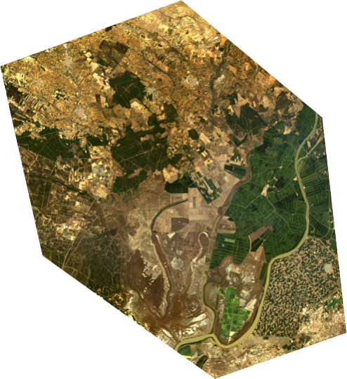
Here we show example of accessing different Landsat mission images, with the AOI in Spain, and we stored it as a Geojson file.
import requests
# Landsat 5
base = 'https://storage.googleapis.com/gcp-public-data-landsat/'
tile = 'LT05/01/202/034/LT05_L1TP_202034_20110905_20161006_01_T1/'
bands = ['LT05_L1TP_202034_20110905_20161006_01_T1_B%d.TIF'%i for i in [1,2,3,4,5,7]]
metadata = requests.get(base + tile + 'LT05_L1TP_202034_20110905_20161006_01_T1_MTL.txt').content.decode()
scale = []
off = []
for i in metadata.split('\n'):
if 'REFLECTANCE_ADD_BAND' in i:
print(i)
off.append(float(i.split(' = ')[1]))
if 'REFLECTANCE_MULT_BAND' in i:
print(i)
scale.append(float(i.split(' = ')[1]))
rgb = []
for i in [0,1,2]:
g = gdal.Warp('', '/vsicurl/' + base + tile + bands[i], format = 'MEM', warpOptions = \
['NUM_THREADS=ALL_CPUS'],srcNodata = 0, dstNodata=0, cutlineDSName= 'aoi.json', \
cropToCutline=True, resampleAlg = gdal.GRIORA_NearestNeighbour)
rgb.append(g.ReadAsArray())
rgb = np.array(scale[:3])[...,None, None]*rgb + np.array(off[:3])[...,None, None]
alpha = np.any(rgb < 0, axis=0)
REFLECTANCE_MULT_BAND_1 = 1.2582E-03
REFLECTANCE_MULT_BAND_2 = 2.6296E-03
REFLECTANCE_MULT_BAND_3 = 2.2379E-03
REFLECTANCE_MULT_BAND_4 = 2.7086E-03
REFLECTANCE_MULT_BAND_5 = 1.8340E-03
REFLECTANCE_MULT_BAND_7 = 2.5458E-03
REFLECTANCE_ADD_BAND_1 = -0.003756
REFLECTANCE_ADD_BAND_2 = -0.007786
REFLECTANCE_ADD_BAND_3 = -0.004746
REFLECTANCE_ADD_BAND_4 = -0.007377
REFLECTANCE_ADD_BAND_5 = -0.007472
REFLECTANCE_ADD_BAND_7 = -0.008371
# since landsat angles has to be produced
# from the angular text file
ang = requests.get(base + tile + 'LT05_L1TP_202034_20110905_20161006_01_T1_ANG.txt').content
with open('landsat/landsat_ang/LT05_L1TP_202034_20110905_20161006_01_T1_ANG.txt', 'wb') as f:
f.write(ang)
header = 'LT05_L1TP_202034_20110905_20161006_01_T1_'
import os
from glob import glob
from multiprocessing import Pool
import subprocess
from functools import partial
cwd = os.getcwd()
#header += cwd
os.chdir('landsat/landsat_ang/')
def translate_angle(band, header):
subprocess.call([cwd+'/util/landsat_angles/landsat_angles', \
header + 'ANG.txt', '-B', '%d'%band])
inp = 'angle_sensor_B%02d.img'%band
oup = header+ 'VZA_VAA_B%02d.TIF'%band
if os.path.exists(oup):
os.remove(oup)
gdal.Translate(oup, inp, creationOptions = \
['COMPRESS=DEFLATE', 'TILED=YES'], noData='-32767').FlushCache()
if not os.path.exists(header + 'SZA_SAA.TIF'):
gdal.Translate(header + 'SZA_SAA.TIF', 'angle_solar_B01.img', creationOptions = \
['COMPRESS=DEFLATE', 'TILED=YES'], noData='-32767').FlushCache()
p = Pool()
par = partial(translate_angle, header=header)
p.map(par, range(1,8))
list(map(os.remove, glob('angle_s*_B*.img*')))
os.chdir(cwd)
sza, saa = gdal.Warp('', 'landsat/landsat_ang/'+ header + 'SZA_SAA.TIF',format = 'MEM', warpOptions = \
['NUM_THREADS=ALL_CPUS'],srcNodata = 0, dstNodata=0, cutlineDSName= 'aoi.json', \
cropToCutline=True, resampleAlg = gdal.GRIORA_NearestNeighbour).ReadAsArray()/100.
rgb = rgb / np.cos(np.deg2rad(sza))
rgb[rgb<0] = np.nan
rgba = np.r_[rgb, ~alpha[None, ...]]
plt.figure(figsize=(8,8))
plt.imshow(rgba.transpose(1,2,0)*2)
<IPython.core.display.Javascript object>

<matplotlib.image.AxesImage at 0x7fae7aa1cf60>
# We save all the remote file to local
# also convert it to reflectance...
for i in range(6):
g = gdal.Warp('', '/vsicurl/' + base + tile + bands[i], format = 'MEM', warpOptions = \
['NUM_THREADS=ALL_CPUS'],srcNodata = 0, dstNodata=0, cutlineDSName= 'aoi.json', \
cropToCutline=True, resampleAlg = gdal.GRIORA_NearestNeighbour)
data = (g.ReadAsArray() * scale[i] + off[i])/np.cos(np.deg2rad(sza))
data[data<0] = -9999
driver = gdal.GetDriverByName('GTiff')
ds = driver.Create('landsat/' + bands[i], data.shape[1], data.shape[0], 1, \
gdal.GDT_Float32, options=["TILED=YES", "COMPRESS=DEFLATE"])
ds.SetGeoTransform(g.GetGeoTransform())
ds.SetProjection(g.GetProjectionRef())
ds.GetRasterBand(1).WriteArray(data)
ds.FlushCache()
ds=None
g = gdal.Warp('landsat/' + bands[0].replace('B1', 'BQA'), '/vsicurl/' + base + tile + bands[0].replace('B1', 'BQA'), format = 'GTiff', warpOptions = \
['NUM_THREADS=ALL_CPUS'],srcNodata = 0, dstNodata=0, cutlineDSName= 'aoi.json', \
cropToCutline=True, resampleAlg = gdal.GRIORA_NearestNeighbour, creationOptions \
= ['COMPRESS=DEFLATE', 'TILED=YES'])
g.FlushCache()
aoi_mask = np.isnan(data)
plt.imshow(gdal.Open('landsat/LT05_L1TP_202034_20110905_20161006_01_T1_B1.TIF').ReadAsArray())
plt.colorbar()
<IPython.core.display.Javascript object>

<matplotlib.colorbar.Colorbar at 0x7fadf404d7b8>
We now have the angle and reflectance for this AOI, we can pass them into SIAC to run the atmospheric correction.
Run SIAC
In reality, we need the emulators for this sensor, but at the moment we do not have, so we instead use Landsat 8 emultors just for demostration purporse.
import numpy as np
from SIAC.the_aerosol import solve_aerosol
from SIAC.the_correction import atmospheric_correction
sensor_sat = 'OLI', 'L8'
toa_bands = ['landsat/'+i for i in bands]
view_angles = ['landsat/landsat_ang/LT05_L1TP_202034_20110905_20161006_01_T1_VZA_VAA_%s.TIF'%i \
for i in ['B01', 'B02', 'B03', 'B04', 'B05', 'B07']]
sun_angles = 'landsat/landsat_ang/LT05_L1TP_202034_20110905_20161006_01_T1_SZA_SAA.TIF'
cloud_mask = gdal.Open('landsat/' + bands[0].replace('B1', 'BQA')).ReadAsArray()
cloud_mask = ~((cloud_mask >= 672) & ( cloud_mask <= 684)) | aoi_mask
band_wv = [469, 555, 645, 859, 1640, 2130]
obs_time = datetime(2011, 9, 5, 10, 51, 11)
#get_mcd43(toa_bands[0], obs_time, mcd43_dir = './MCD43/', vrt_dir = './MCD43_VRT')
band_index = [1,2,3,4,5,6]
aero = solve_aerosol(sensor_sat,toa_bands,band_wv, band_index,\
view_angles,sun_angles,obs_time,cloud_mask,aot_prior = 0.05, \
aot_unc=0.1, mcd43_dir= './MCD43_VRT/',gamma=10., ref_scale = 1., ref_off = 0., a_z_order=0)
aero._solving()
base = 'landsat/LT05_L1TP_202034_20110905_20161006_01_T1_'
aot = base + 'aot.tif'
tcwv = base + 'tcwv.tif'
tco3 = base + 'tco3.tif'
aot_unc = base + 'aot_unc.tif'
tcwv_unc = base + 'tcwv_unc.tif'
tco3_unc = base + 'tco3_unc.tif'
rgb = [toa_bands[2], toa_bands[1], toa_bands[0]]
atmo = atmospheric_correction(sensor_sat, toa_bands, band_index,view_angles,sun_angles, \
aot = aot, cloud_mask = cloud_mask, tcwv = tcwv, tco3 = tco3, \
aot_unc = aot_unc, tcwv_unc = tcwv_unc, tco3_unc = tco3_unc, \
rgb = rgb, ref_scale = 1., ref_off = 0., a_z_order = 0)
ret = atmo._doing_correction()
2018-09-13 18:41:35,579 - AtmoCor - INFO - Set AOI.
2018-09-13 18:41:35,581 - AtmoCor - INFO - Get corresponding bands.
2018-09-13 18:41:35,581 - AtmoCor - INFO - Slice TOA bands based on AOI.
2018-09-13 18:41:36,815 - AtmoCor - INFO - Parsing angles.
2018-09-13 18:41:36,821 - AtmoCor - INFO - Mask bad pixeles.
2018-09-13 18:41:37,122 - AtmoCor - INFO - Get simulated BOA.
2018-09-13 18:42:25,089 - AtmoCor - INFO - Get PSF.
2018-09-13 18:42:28,284 - AtmoCor - INFO - Solved PSF: 8.67, 11.33, 0, 4, 1, and R value is: 0.961.
2018-09-13 18:42:28,288 - AtmoCor - INFO - Get simulated TOA reflectance.
2018-09-13 18:42:31,141 - AtmoCor - INFO - Filtering data.
2018-09-13 18:42:31,199 - AtmoCor - INFO - Loading emulators.
2018-09-13 18:42:33,766 - AtmoCor - INFO - Reading priors and elevation.
2018-09-13 18:42:42,059 - MultiGrid solver - INFO - MultiGrid solver in process...
2018-09-13 18:42:42,060 - MultiGrid solver - INFO - Total 5 level of grids are going to be used.
2018-09-13 18:42:42,061 - MultiGrid solver - INFO - [94mOptimizing at grid level 1
+++++++++++++++++++++++++++++++++++++++++++++++++++++++++++++++++++++++++++++++++++++++++++++++++++++++++
2018-09-13 18:42:43,462 - MultiGrid solver - INFO - [92mb'CONVERGENCE: REL_REDUCTION_OF_F_<=_FACTR*EPSMCH'
2018-09-13 18:42:43,463 - MultiGrid solver - INFO - [92mIterations: 4
2018-09-13 18:42:43,463 - MultiGrid solver - INFO - [92mFunction calls: 23
2018-09-13 18:42:43,464 - MultiGrid solver - INFO - [94mOptimizing at grid level 2
+++++++++++++++++++++++++++++++++++++++++++++++++++++++++++++++++++++++++++++++++++++++++++++++++++++++++
2018-09-13 18:42:46,115 - MultiGrid solver - INFO - [92mb'CONVERGENCE: REL_REDUCTION_OF_F_<=_FACTR*EPSMCH'
2018-09-13 18:42:46,116 - MultiGrid solver - INFO - [92mIterations: 3
2018-09-13 18:42:46,116 - MultiGrid solver - INFO - [92mFunction calls: 25
2018-09-13 18:42:46,117 - MultiGrid solver - INFO - [94mOptimizing at grid level 3
+++++++++++++++++++++++++++++++++++++++++++++++++++++++++++++++++++++++++++++++++++++++++++++++++++++++++
2018-09-13 18:42:57,283 - MultiGrid solver - INFO - [92mb'STOP: TOTAL NO. of f AND g EVALUATIONS EXCEEDS LIMIT'
2018-09-13 18:42:57,283 - MultiGrid solver - INFO - [92mIterations: 8
2018-09-13 18:42:57,284 - MultiGrid solver - INFO - [92mFunction calls: 75
2018-09-13 18:42:57,284 - MultiGrid solver - INFO - [94mOptimizing at grid level 4
+++++++++++++++++++++++++++++++++++++++++++++++++++++++++++++++++++++++++++++++++++++++++++++++++++++++++
2018-09-13 18:43:09,654 - MultiGrid solver - INFO - [92mb'CONVERGENCE: REL_REDUCTION_OF_F_<=_FACTR*EPSMCH'
2018-09-13 18:43:09,655 - MultiGrid solver - INFO - [92mIterations: 10
2018-09-13 18:43:09,655 - MultiGrid solver - INFO - [92mFunction calls: 36
2018-09-13 18:43:09,656 - MultiGrid solver - INFO - [94mOptimizing at grid level 5
+++++++++++++++++++++++++++++++++++++++++++++++++++++++++++++++++++++++++++++++++++++++++++++++++++++++++
2018-09-13 18:45:07,040 - MultiGrid solver - INFO - [92mb'CONVERGENCE: REL_REDUCTION_OF_F_<=_FACTR*EPSMCH'
2018-09-13 18:45:07,040 - MultiGrid solver - INFO - [92mIterations: 10
2018-09-13 18:45:07,041 - MultiGrid solver - INFO - [92mFunction calls: 32
2018-09-13 18:45:10,977 - AtmoCor - INFO - Finished retrieval and saving them into local files.
2018-09-13 18:45:13,309 - AtmoCor - INFO - Set AOI.
2018-09-13 18:45:13,310 - AtmoCor - INFO - Slice TOA bands based on AOI.
2018-09-13 18:45:14,708 - AtmoCor - INFO - Parsing angles.
2018-09-13 18:45:15,728 - AtmoCor - INFO - Parsing auxs.
2018-09-13 18:45:16,584 - AtmoCor - INFO - Parsing atmo parameters.
2018-09-13 18:45:23,338 - AtmoCor - INFO - Loading emus.
2018-09-13 18:45:25,858 - AtmoCor - INFO - Get correction coefficients.
2018-09-13 18:45:32,039 - AtmoCor - INFO - Doing corrections.
2018-09-13 18:45:37,474 - AtmoCor - INFO - Composing RGB.
2018-09-13 18:45:39,423 - AtmoCor - INFO - Done.
TOA image |
BOA image |
|---|---|
|
|

toa = []
boa = []
for i in range(6):
toa.append(gdal.Open(toa_bands[i]).ReadAsArray(1500, 500, 1,1)[0,0])
boa.append((gdal.Open(toa_bands[i].replace('.TIF', '_sur.tif')).ReadAsArray(1500, 500, 1,1)[0,0])/10000.)
plt.plot(band_wv, toa, 's-', label='TOA')
plt.plot(band_wv, np.array(boa), 'o-', label='BOA')
plt.legend()
<IPython.core.display.Javascript object>

<matplotlib.legend.Legend at 0x7fade5894080>
Here we demonstrate the use of SIAC for the correction of Landsat 5 images, but it can only treated as a test and if one wants to do the real AC of Landsat 5 collection, the emulators and spectral mapping should be created for Landsat 5 TM sensor also a more resonable prior should be used.
Indices and tables
MULTIPLY - SAR Pre Processing
Introduction
Scope
The MULTIPLY project will “develop a new platform for joint and consistent retrieval of Copernicus SENTINEL data and beyond”. This document presents the Algorithm Theoretical Basis Document (ATBD) of the MULTIPLY project. The ATBD aims at providing a detailed description of the algorithms implemented in the different processing chains, including a scientific background, a justification for each implemented algorithm and the parameterisation used in the project. This ATBD is written through successive increments. This initial version (v1) deals with the coarse resolution data in general. The second version focus on the activities regarding the high- resolution data and a last version (v3) will be released at the end of the project. The ATBD-v3 will be the final version of the document.
Structure of this documentation
Need to be done !!!
This documentation gives a detailed
The documentation is organised in ... main sections.
- Section
- Section
- Section
Installation
The standard python way
You can download the source code from the project website. Unpack the file you obtained and then run:
python setup.py install
Using conda
not yet implemented
Using pip
not yet implemented
From code repository for developing
to be continued
Installation from the recent stable code repository can be done by:
to be continued
Processing Chain
put "Sentinel-1 Level-1 SLC data" in the caption? Depends on other parts!
How will the deliverable be organized?
Overview
The two Sentinel-1 satellites 1A and 1B are one of the first satellites which are providing microwave data in high temporal and spatial resolution. Within the MULTIPLY project we developed a preprocessing chain to process time-series of Sentinel-1 data for quantitative analysis of vegetation and soil parameters over agricultural fields. Therefore, rigorous geometric and radiometric corrections as well as a multi-temporal speckle filter is applied. The different preprocessing steps are shown in Fig. 2 and Fig. 3. Furthermore, every processing step is explained in more detail in the following subsections. As it can be seen Fig. 2 and Fig. 3 the preprocessing work-flow is split in two main parts. The preprocessing methods in Fig. 2 can be applied separately for every image. Whereas the work-flow shown in Fig. 3 need several images which were preprocessed by the different steps presented in Fig. 2.
The whole preprocessing chain for Sentinel-1 Level-1 Single Look Complex (SLC) data is accomplished by ESA’s SNAP S1TBX software (current version 5.0.4). The SNAP toolbox can be downloaded from http://step.esa.int/main/download/. However, to automatically apply different preprocessing steps on Sentinel-1 data a python script, which uses the Graph Processing Tool (GPT) of the S1TBX, is provided. All codes, xml-graphs etc are stored in a GitHub repository accessible under https://github.com/multiply-org/sar-pre-processing.

First main part of the used preprocessing chain (rigorous geometric and radiometric correction including preliminary operations)

Second main part of the used preprocessing chain (Co-registration and multi-temporal speckle filter)
Sentinel-1 Level-1 SLC data
The preprocessing work-flow of Fig. 2 is based on Sentinel-1 Level-1 SLC data. Among some other sources Sentinel-1 data can be downloaded from ESA’s Copernicus Open Access Hub (https://scihub.copernicus.eu/).
Sentinel-1 Level-1 SLC data are generated by the operational ESA Instrument Processing Facility (IPF). The SLC products are situated in slant range geometry. The slant range geometry is the natural radar one and is defined by the line-of-sight distance of the radar system to each reflecting object. The SLC product consists of focused SAR data in zero-Doppler orientation. Furthermore, for geo-referencing orbit and attitude information directly provided by the satellite are stored within the SLC product. Moreover the SAR data is corrected for errors caused by the well known azimuth bi-static delay, elevation antenna pattern and range spreading loss [1]. In contrary to Level-1 Ground Range Detected (GRD) products SLC data preserve the real and imaginary part of the backscatter signal and contain therefore also the phase information [1]. The IPF is generating SLC data for all available acquisition modes (StripMap (SM), Interferometric Wide (IW), Extra Wide (EW), and Wave (WV)) of the Sentinel-1 satellites. Further information about Sentinel-1 Level-1 products are gathered in ESA’s Sentinel-1 User Handbook [1] available at https://earth.esa.int/documents/247904/685163/Sentinel-1_User_Handbook.
Precise orbit file
Theory / Purpose
During the acquisition of Sentinel-1 data the satellite position is recorded by a Global Navigation Satellite System (GNSS). To assure a fast delivery of Sentinel-1 products orbit information generated by an on-board navigation solution are stored within the Sentinel-1 Level-1 products. The orbit positions are later refined and made available as restituted or precise orbit files by the Copernicus Precise Orbit Determination (POD) Service. The POD products for Sentinel-1 data with given accuracy and availability after data acquisition are listed in Table 1.
Mission |
POD Product |
Accuracy |
Latency |
Sentinel-1 |
Restituted Orbit File |
< 10 cm |
3 hours |
Precise Orbit Ephemerides (POE) Orbit file |
< 5 cm |
20 days |
|
Attitude Restituted Data |
< 0.005 deg |
20 days |
Precise orbit information can have a high influence on the quality of several preprocessing steps especially e.g. for the geo-referencing of the data. Therefore, it is always preferable to use the most accurate orbit information that is available.
Practical implementation
Since the preprocessing for the MULTIPLY project doesn’t depend on near-real-time data the precise orbit file (available within 20 days) is used to update the orbit and velocity information within the Sentinel-1 SLC product. Therefore the operator “Apply Orbit Correction” of SNAP S1TBX toolbox is used.
- Input:
Sentinel-1 SLC IW image (downloaded from Copernicus Open Access Hub)
Precise orbit file (automatic download by SNAP S1TBX)
- Output:
Sentinel-1 SLC IW image with updated orbit information
Thermal noise removal
Theory / Purpose
Thermal noise is caused by the background energy of a SAR receiver and independent from the received signal power. Like some other noise factors thermal noise appears randomly over the entire image. But in contrary to quantization noise like speckle, which is connected to the signal power, thermal noise is hardly noticeable. Therefore, high impact of thermal noise on the quality of the data is especially given in areas like calm lakes, rivers and other with a low mean signal response detected by the SAR system. For the purpose of correction the IPF is calculating a thermal noise Look up Table (LUT) which is stored within the Sentinel-1 Level-1 product. More information about the calculation of the thermal noise for Sentinel-1 is given in [3].
Practical implementation
The “Thermal Noise Removal” operator of SNAP S1TBX software is used to remove the thermal noise which is stored within a LUT within Sentinel-1 Level-1 products. Thermal noise removal can only applied on backscatter intensity therefore the phase information of the SLC data get lost.
- Input:
Sentinel-1 SLC IW image with updated orbit information
- Output:
Sentinel-1 SLC Intensity corrected by thermal noise
Radiometric calibration
Theory / Purpose
Sentinel-1 Level-1 products are not radiometric corrected by default. However, for the quantitative use of SAR images a radiometric calibration of radar reflectivity (stored as Digital Numbers (DN) within Sentinel-1 Level-1 products) to physical units (radar backscatter) is essential. Otherwise a comparison of SAR images from different sensors or even the same sensor for different acquisition dates or different acquisition modes is not possible. To apply a radiometric calibration a Calibration Annotation Data Set (CADS) with four Look Up Tables (LUTs) are provided within the Sentinel-1 Level-1 products by Sentinel-1 Instrument Processing Facility (IPF). The four LUTs are used to convert DN to sigma naught, beta naught and gamma or vice versa. More information about the radiometric calibration is given in [4].
Practical implementation
The “Radiometric Calibration” operator of SNAP S1TBX software is used to perform the conversion of DN to radar backscatter. In our case the output radar backscatter information is calibrated in Sigma naught.
- Input:
Sentinel-1 SLC Intensity corrected by thermal noise
- Output:
Sigma naught calibrated radar backscatter
TOPSAR Deburst
Theory / Purpose
Sentinel-1 Level-1 SLC images acquired in IW or EW swath mode consists of one image per swath and polarisation. IW products are made up of three swaths which means three images for single polarisation and six images for dual polarisation. EW products are made up of five swaths which means five images for single polarisation and ten images for dual polarisation. The sub-swath images consists of different bursts which are all processed as separate images. The different bursts are stored in one single image whereby each burst is separated by a black-filled demarcation [1]. For the usage of Sentinel-1 Level-1 SLC data only one sub-swath can be extracted or several/all sub-swath can be combined to one image with fluent transitions between the sub-swaths. More detailed information are provided in [1], [5] and [6].
Practical implementation
The “TOPSAR-Deburst” operator of SNAP S1TBX software is used to merge all sub-swath to retrieve one fluent image.
- Input:
Sigma naught calibrated radar backscatter (with different sub-swath)
- Output:
Sigma naught calibrated radar backscatter (with fluent transitions)
Geometric correction
Theory / Purpose
An important part of the preprocessing chain is the geometric terrain correction. The geometric correction is a conversion of the Sentinel-1 SLC data from slant range geometry into a map coordinate system. Due to the acquisition geometry of the SAR different topographical distortions like foreshortening, layover or shadowing effects occur. The appropriate way to correct these distortions is the Range-Doppler approach. The method needs information about the topography (normally provided by a Digital Elevation Model (DEM)) as well as orbit and velocity information from the satellite (stored within Sentinel-1 SLC product) to correct the mentioned distortions and derive a precise geolocation for each pixel of the image.
Practical implementation
A geometric correction of the input data is performed by using the “Range Doppler Terrain Correction” method implement in SNAP’s S1TBX software. Data from the Shuttle Radar Topography Mission (SRTM) with a resolution of 1-arc second (30 meters) is used for the necessary DEM.
- Input:
Sigma naught calibrated radar backscatter (with fluent transitions)
SRTM data with 1-arc second resolution (automatic download by SNAP S1TBX)
- Output:
Geometric corrected sigma naught calibrated radar backscatter (Map Projection WGS84)
Incidence angle from ellipsoid
Local incidence angle (based on SRTM)
Radiometric correction
Theory / Purpose
For the conversion of Sentinel-1 backscatter values to sigma or gamma naught, LUT’s stored within the Sentinel-1 product are used (see Radiometric calibration). For the creation of the LUT’s Sentinel-1 IPF is using an incidence angle of an ellipsoid inflated earth model [4]. Therefore, the local terrain variation within the image and their radiometric impact on the backscatter is considered insufficiently. A simple and widely used practice to consider the radiometric impact due to local terrain variations represents the approach to use the local incidence angle instead of the ellipsoid one [7]. The radiometric corrected backscatter \(\sigma_{NORLIM}^{0}\) used by Kellndorfer et al. [7] can be calculated as
with \(\theta_{LIA}\) as the local incidence angle, \(\theta_{Ell}\) as the ellipsoid incidence angle used by IPF and the radar backscatter \(\sigma_{Ell}\) calculated by using LUT’s provided by IPF.
Practical implementation
Within the “Range Doppler Terrain Correction” method of SNAP’s S1TBX software the radiometric normalisation approach of Kellndorfer et al. [7] is implemented as a additional option. Unfortunately, the SNAP internal option can not be used with our kind of data. Therefore, normalisation after Kellndorfer et al [7] is done by coding the equations within the “BandMath” operator of SNAP’s S1TBX. The used local incidence angle is provided by the previous applied “Range Doppler Terrain Correction” and therefore the local incidence angle is based on the SRTM data.
- Input:
Geometric corrected sigma naught calibrated radar backscatter (Map Projection WGS84)
Incidence angle from ellipsoid
Local incidence angle (based on SRTM)
- Output:
Radiometric and geometric corrected sigma naught calibrated radar backscatter (Map Projection WGS84)
Backscatter normalisation
Theory / Purpose
Beside the previously discussed geometric and radiometric distortions some other specific backscattering coefficient variations within the range direction of the image are caused by the image geometry of the SAR sensor. The backscattered energy of an illuminated area has not only a dependency on the area itself but also on the incidence angle. This means, backscatter values of a specific area with a small incidence angle return higher backscatter values then data of the same area acquired with a higher incidence angle. Incidence angle induced variations not only occur inside one image but also between images form different sensors as well as within one sensor through different acquisition geometries or different tracks or orbits. For a usage of Sentinel-1A and 1B time-series acquired with different orbits and/or different tracks and therefore most likly a high change between the incidence angles a backscatter normalisation is vital. A often and widely used technique to minimize backscatter variations caused by the incidence angle is the cosine correction [8]. The cosine correction is based on the Lambert’s law for optics. Therefore, under the assumption that the backscattered energy in the upper hemisphere follows a cosine law and also the radiation variability has a cosine dependency, the received backscatter \(\sigma_{\theta_i}^{0}\) and its dependency on the incidence angle can be written as
with a weighting factor n and the incidence angle independent backscatter \(\sigma_{0}^{0}\). With the cosine correction the backscatter of the Sentinel-1 products can therefore normalised to a reference angle \(\theta_{ref}\) with
Studies show that the weighting factor n is dependent on the roughness [9] and therefore the backscatter variations can vary with different land cover types. A schematic illustration of the backscatter variations considering the incidence angle is given in Fig. 4.

Practical implementation
The backscatter normlisation is applied by coding (3) in SNAP’s S1TBX operator “BandMaths”. As default a reference angle of 37,55° (average incidence angle for IW swath mode [3]) and a weighting factor of 2 (standard value) is specified. Through a configuration file the user can replace the default values for the reference angle and weighting factor to probably more suitable values of their specific applications.
- Input:
Radiometric and geometric corrected sigma naught calibrated radar backscatter (Map Projection WGS84)
reference angle (default is 37,55°)
weighting factor (default is 2)
- Output:
Radiometric and geometric corrected sigma naught calibrated radar backscatter values normalised to reference angle (Map Projection WGS84)
Co-registration
Theory / Purpose
For time-series analysis especially when applying a Multi-temporal speckle filter the SAR image has to be co-registered. The co-registration is a method to get every image of the time-series on the same grid and also the pixel resolution.
Practical implementation
The co-registration as a requirement for the Multi-temporal speckle filter is accomplished by the “Co-Registration” operator within SNAP’s S1TBX. The “Co-Registration” operator in SNAP is defined as a completely automatic process. The operator consists of a stack creation (collocating master and slave image), a cross correlation (allignment between master ans slave image) and a warp (resamples pixels from the slave image to pixels of the master image).
- Input:
Master image
Slave image(s)
- Output:
Co-registered images
Multi-temporal speckle filter
Theory / Purpose
A characteristic of images acquired by a SAR system is the visibility of random noise which look like “salt and pepper” within the image and is called speckle. The appearance of speckle is caused by the interferences of coherent echoes from individual scatterers within one pixel [11].The presence of speckle degrades the quality of the image and therefore it makes the interpretation of the SAR data more difficult. Over the years several approaches for speckle reduction were developed. They are mainly based on either multi-looking or filtering methods. Different filtering approaches like Frost, Lee etc. can be applied as a single or multi-temporal speckle filter. First findings with Sentinel-1 data show that a multi-temporal speckle filter provides better results in form of speckle reduction and resolution preservation then a single speckle filter. A major advantage for the usage of a multi-temporal speckle filter on Sentinel-1 data is the high temporal resolution availability. Nevertheless, more detailed studies on analysing the impact of different multi-temporal speckle filters on the retrieval of bio- and geophysical parameters from Sentinel-1 data are still lacking. Anyway, a usage of a multi-temporal filter significantly reduces the speckle and is therefore a essentinal part of our preprocessing chain.
Practical implementation
For the speckle reduction the “Multi-temporal Speckle Filter” operator within SNAP’s S1TBX software is used. Currently 15 temporally consecutive images are used within the “Multi-temporal Speckle Filter” whereby the target image is temporally situated in the middle. The applied filter is a Lee filter with spatial averaging over 3x3 pixel. The spatial averaging over pixel has a significant influence on spatial resolution information loss of the image. Therefore, the averaging pixel size might change during the project. If the image consists of two polarisations the filter is applied on each polarisation separately. The practical implementation in case of filter type, used polarisation, number of used images etc. may change with more experience of applying multi-temporal speckle filters and the occurring results.
- Input:
15 co-registered images
- Output:
speckle filtered images
References
- 1(1,2,3,4,5)
Sentinel-1 Team. Sentinel-1 user handbook. Manual, ESA, Ref: GMES-S1OP-EOPG-TN-13-0001, 2013.
- 2
Sentinels POD team. Sentinels pod service file format specifications. Technical Report, ESA, Ref: GMES-GSEG-EOPG-FS-10-0075, 2016.
- 3(1,2)
H. Bourbigot, H. Johnsen, and Piantanida R. Sentinel-1 product definition. Technical Report, ESA, Ref: S1-RS-MDA-53-7440, 2015.
- 4(1,2)
N. Miranda and P.J. Meadows. Radiometric calibration of s-1 level-1 products generated by the s-1 ipf. Technical Report, ESA, Ref: ESA-EOPG-CSCOP-TN-0002, 2015.
- 5
D d’Aria, F De Zan, D Giudici, A Monti Guarnieri, and F Rocca. Burst-mode sars for wide-swath surveys. Canadian Journal of Remote Sensing, 33(1):27–38, 2007.
- 6
Francesco De Zan and AM Monti Guarnieri. Topsar: terrain observation by progressive scans. IEEE Transactions on Geoscience and Remote Sensing, 44(9):2352–2360, 2006.
- 7(1,2,3,4)
J. M. Kellndorfer, L. E. Pierce, M. C. Dobson, and F. T. Ulaby. Toward consistent regional-to-global-scale vegetation characterization using orbital sar systems. IEEE Transactions on Geoscience and Remote Sensing, 36(5):1396–1411, Sep 1998. doi:10.1109/36.718844.
- 8
Fawwaz T Ulaby, Richard K Moore, and Adrian K Fung. Microwave remote sensing: active and passive. Vol. 2, Radar remote sensing and surface scattering and emission theory. Addison-Wesley Reading, MA, 1982.
- 9
J. P. Ardila, V. Tolpekin, and W. Bijker. Angular backscatter variation in l-band alos scansar images of tropical forest areas. IEEE Geoscience and Remote Sensing Letters, 7(4):821–825, Oct 2010. doi:10.1109/LGRS.2010.2048411.
- 10
W. Wagner, G. Lemoine, M. Borgeaud, and H. Rott. A study of vegetation cover effects on ers scatterometer data. IEEE Transactions on Geoscience and Remote Sensing, 37(2):938–948, Mar 1999. doi:10.1109/36.752212.
- 11
Iain H Woodhouse. Introduction to microwave remote sensing. CRC press, 2005.
Technical documentation
Sar-Pre-Processing
Wrapper module to launch preprocessor
-
class
sar_pre_processing.sar_pre_processor.AttributeDict(**entries)[source]¶ Bases:
objectA class to convert a nested Dictionary into an object with key-values accessibly using attribute notation (AttributeDict.attribute) instead of key notation (Dict[“key”]). This class recursively sets Dicts to objects, allowing you to recurse down nested dicts (like: AttributeDict.attr.attr)
-
class
sar_pre_processing.sar_pre_processor.SARPreProcessor(**kwargs)[source]¶ Bases:
sar_pre_processing.sar_pre_processor.PreProcessor-
pre_process_step1(**kwargs)[source]¶ Pre-process S1 SLC data with SNAP’s GPT
apply precise orbit file
thermal noise removal
calibration
TOPSAR-Deburst
Geometric Terrain Correction
Radiometric Correction (after kellndorfer et al.)
backscatter normalisation on specified angle in config file (based on Lambert’s Law)
-
File list for Sar-Pre-Processing
Create List of SAR data which will be processed by sar_pre_processer module
-
class
sar_pre_processing.file_list_sar_pre_processing.AttributeDict(**entries)[source]¶ Bases:
objectA class to convert a nested Dictionary into an object with key-values accessibly using attribute notation (AttributeDict.attribute) instead of key notation (Dict[“key”]). This class recursively sets Dicts to objects, allowing you to recurse down nested dicts (like: AttributeDict.attr.attr)
Thomas weiß <”weiss.thomas@lmu.de”>
MULTIPLY - Forward Operators
A suggestion for a structure is
introduction
concepts / algorithm
user manual
architecture
api reference
Emulators for complex models using Gaussian Processes in Python: gp_emulator
The gp_emulator library provides a simple pure Python implementations of Gaussian Processes (GPs), with a view of using them as emulators of complex computers code. In particular, the library is focused on radiative transfer models for remote sensing, although the use is general. The GPs can also be used as a way of regressing or interpolating datasets.
If you use this code, please cite both the code and the paper that describes it.
JL Gómez-Dans, Lewis PE, Disney M. Efficient Emulation of Radiative Transfer Codes Using Gaussian Processes and Application to Land Surface Parameter Inferences. Remote Sensing. 2016; 8(2):119. DOI:10.3390/rs8020119
José Gómez-Dans & Professor Philip Lewis. (2018, October 12). jgomezdans/gp_emulator (Version 1.6.5). Zenodo. DOI:10.5281/zenodo.1460970
Development of this code has received funding from the European Union’s Horizon 2020 research and innovation programme under grant agreement No 687320, under project H2020 MULTIPLY.
Gaussian Process Emulators
Introduction
Often, complex and numerically demanding computer codes are required in inverse modelling tasks. Such models might need to be invoked repeatedly as part of a minimisition task, or in order to provide some numerically-integrated quantity. This results in many applications being rendered impractical as the codes are too slow.
The concept of an emulator is simple: for a given model, let’s provide a function that given the same inputs are the original model, gives the same output. Clearly, we need to qualify “the same”, and maybe downgrade the expectations to “a very similar output”. Ideally, with some metric of uncertainty on the prediction. So an emulator is just a fast, surrogate to a more established code.
Gaussian processes (GPs) have been used for this task for years, as they’re very flexible throught he choice of covariance function that can be used, but also work remarkably well with models that are nonlinear and that have a reasonable number of inputs (10s).
We have used these techniques for emulation radiative transfer models used in Earth Observation, and we even wrote a nice paper about it: Gomez-Dans et al (2016). Read it, it’s pure gold.
Installing the package
The package works on Python 3. With a bit of effort it’ll probably work on Python 2.7. The only dependencies are scipy and numpy To install, use either conda:
conda install -c jgomezdans gp_emulator
or pip:
pip install gp_emulator
or just clone or download the source repository and invoke setup.py script:
python setup.py install
Quickstart
Single output model emulation
Assume that we have two arrays, X and y. y is of size N, and it stores the N expensive model outputs that have been produced by running the model on the N input sets of M input parameters in X. We will try to emulate the model by learning from these two training sets:
gp = gp_emulator.GaussianProcess(inputs=X, targets=y)
Now, we need to actually do the training…
gp.learn_hyperparameters()
Once this process has been done, you’re free to use the emulator to predict the model output for an arbitrary test vector x_test (size M):
y_pred, y_sigma, y_grad = gp.predict (x_test, do_unc=True,
do_grad=True)
In this case, y_pred is the model prediction, y_sigma is the variance associated with the prediction (the uncertainty) and y_grad is an approximation to the Jacobian of the model around x_test.
Let’s see a more concrete example. We create a damped sine, add a bit of Gaussian noise, and then subsample a few points (10 in this case), fit the GP, and predict the function over the entire range. We also plot the uncertainty from this prediction.
We can see that the GP is doing an excellent job in predicting the function, even in the presence of noise, and with a handful of sample points. In situations where there is extrapolation, this is indicated by an increase in the predictive uncertainty.
Multiple output emulators
In some cases, we can emulate multiple outputs from a model. For example, hyperspectral data used in EO can be emulated by employing the SVD trick and emulating the individual principal component weights. Again, we use X and y. y is now of size N, P, and it stores the N expensive model outputs (size P) that have been produced by running the model on the N input sets of M input parameters in X. We will try to emulate the model by learning from these two training sets, but we need to select a variance level for the initial PCA (in this case, 99%)
gp = gp_emulator.MultivariateEmulator (X=y, y=X, thresh=0.99)
Now, we’re ready to use on a new point x_test as above:
y_pred, y_sigma, y_grad = gp.predict (x_test, do_unc=True,
do_grad=True)
A more concrete example: let’s produce a signal that can be decomposed as a sum of scaled orthogonal basis functions…
Emulating a typical radiative transfer model
This package was designed to emulate radiatie transfer models. The process entails the following steps:
Decide on what input parameters are required
Decide their ranges
Generate a training input parameter set
Run the model for each element of the input training set and store the outputs
Pass the input and output training pairs to the library, and let it fit the hyperparameters
We can show how this works with an example of the PROSPECT+SAIL model.
Setting the input parameter ranges
We can set the parameter names and their ranges simply by having lists with minimum and maximum values. This assumes a uniformly-distributed parameter distribution between those two boundaries, but other distributions are possible (we never had any reason to try them though!). We additionally set up the SRFs and other variables that need to be defined here… We train the model on 250 samples and test on (say) 100. 100 validation samples is probably too few, but for the sake of not waiting too much… ;-)
from functools import partial
import numpy as np
import gp_emulator
import prosail
# Spectral band definition. Just a top hat, with start and
# end wavlengths as an example
b_min = np.array( [ 620., 841, 459, 545, 1230, 1628, 2105] )
b_max = np.array( [ 670., 876, 479, 565, 1250, 1652, 2155] )
wv = np.arange ( 400, 2501 )
passband = []
# Number of training and validation samples
n_train = 250
n_validate = 100
# Validation number is small, increase to a more realistic value
# if you want
# Define the parameter names and their ranges
# Note that we are working here in transformed coordinates...
# Define geometry. Each emulator is for one geometry
sza = 30.
vza = 0.
raa = 0. # in degrees
parameters = [ 'n', 'cab', 'car', 'cbrown', 'cw', 'cm', 'lai', 'ala', 'bsoil', 'psoil']
min_vals = [ 0.8 , 0.46301307, 0.95122942, 0. , 0.02829699,
0.03651617, 0.04978707, 0.44444444, 0. , 0.]
max_vals = [ 2.5 , 0.998002 , 1. , 1. , 0.80654144,
0.84366482, 0.99501248, 0.55555556, 2. , 1 ]
We then require a function for calling the RT model. In the case of PROSAIL, we can do that easily from Python, in other models available in e.g. Fortran, you could have a function that calls the external model
def inverse_transform ( x ):
"""Inverse transform the PROSAIL parameters"""
x_out = x*1.
# Cab, posn 1
x_out[1] = -100.*np.log ( x[1] )
# Cab, posn 2
x_out[2] = -100.*np.log ( x[2] )
# Cw, posn 4
x_out[4] = (-1./50.)*np.log ( x[4] )
#Cm, posn 5
x_out[5] = (-1./100.)*np.log ( x[5] )
# LAI, posn 6
x_out[6] = -2.*np.log ( x[6] )
# ALA, posn 7
x_out[7] = 90.*x[7]
return x_out
def rt_model ( x, passband=None, do_trans=True ):
"""A coupled land surface/atmospheric model, predicting refl from
land surface parameters. Thisfunction provides estimates of refl for
a particular illumination geometry.
The underlying land surface reflectance spectra is simulated using
PROSAIL. The input parameter ``x`` is a vector with the following components:
* ``n``
* ``cab``
* ``car``
* ``cbrown``
* ``cw``
* ``cm``
* ``lai``
* ``ala``
* ``bsoil``
* ``psoil``
"""
x, sza, vza, raa = x
# Invert parameter LAI
if do_trans:
x = inverse_transform ( x )
################# surface refl with prosail #####################
surf_refl = prosail.run_prosail(x[0], x[1], x[2], x[3], x[4], x[5], x[6], x[7], 0.01, sza, vza, raa,
rsoil=x[8], psoil=x[9])
if passband is None:
return surf_refl
else:
return surf_refl[passband].mean()
Now we loop over all the bands, and prepare the emulators. we do this by using the create_emulator_validation function, that does everything you’d want to do… We just stuff the emulator, training and validation sets in one list for convenience.
retval = []
for iband,bmin in enumerate ( b_min ):
# Looping over the bands....
print("Doing band %d" % (iband+1))
passband = np.nonzero( np.logical_and ( wv >= bmin, wv <= b_max[iband] ) )
# Define the SRF for the current band
# Define the simulator for convenience
simulator = partial (rt_model, passband=passband)
# Actually create the training and validation parameter sets, train the emulators
# and return all that
x = gp_emulator.create_emulator_validation (simulator, parameters, min_vals, max_vals,
n_train, n_validate, do_gradient=True,
n_tries=15, args=(30, 0, 0) )
retval.append (x)
A simple validation visualisation looks like this

Comparison between the simulated output and the corresponding emulator output for the validation dataset. Correlations (R2) are in all cases better than 0.99. Slope was between 0.97 and 1., whereas the bias term was smaller than 0.002.
An spectral emulator of PROSAIL
For the case of a spectral emulator, the approach is the same, only that we just use the spectral emulator, which is a bit simpler.
n_train = 350
n_validate = 100
x = gp_emulator.create_emulator_validation ( rt_model, parameters, min_vals, max_vals,
n_train, n_validate, do_gradient=True,
n_tries=10, args=(30, 0, 0) )
The validation results looks like this:

Distribution of residuals derived from the difference of the emulator and simulator for PROSAIL.
We can also check that the gradient of the model is sensible, by comparing it with finite difference approximations from the original model, which is already carried out by create_emulator_validation if we set the do_gradient option.

Comparison of the emulated model gradient versus finite difference approximation for LAI and chlorophyll at different spectral regions.
GPs as regressors for biophyiscal parameter inversion
GPs are a general regression technique, and can be used to regress some wanted magnitude from a set of inputs. This isn’t as cool as other things you can do with them, but it’s feasible to do… GPs are flexible for regression and interpolation, but given that this library has a strong remote sensing orientation, we’ll consider their use for bionpysical parameter extraction from Sentinel-2 data (for example).
Retrieving bionpysical parameters for Sentinel-2
Let’s assume that we want to retrieve leaf area index (LAI) from Sentinel-2 surface reflectance data. The regression problem can be stated as one where the inputs to the regressor are the spectral measurements of a pixel, and the output is the retrieved LAI. We can do this mapping by pairing in situ measurements, or we can just use a standard RT model to provide the direct mapping, and then learn the inverse mapping using the GP.
Although the problem is easy, we know that other parameters will have an effect in the measuremed reflectance, so we can only expect this to work over a limited spread of parameters other than LAI. Here, we show how to use the gp_emulator helper functions to create a suitable training set, and perform this.
1 2 3 4 5 6 7 8 9 10 11 12 13 14 15 16 17 18 19 20 21 22 23 24 25 26 27 28 29 30 31 32 33 34 35 36 37 38 39 40 41 42 43 44 45 46 47 48 49 50 51 52 53 54 55 56 57 58 59 60 61 62 63 64 65 66 67 68 69 70 71 | import numpy as np
import scipy.stats
import gp_emulator
import prosail
import matplotlib.pyplot as plt
np.random.seed(42)
# Define number of training and validation samples
n_train = 200
n_validate = 500
# Define the parameters and their spread
parameters = ["n", "cab", "car", "cbrown", "cw", "cm", "lai", "ala"]
p_mins = [1.6, 25, 5, 0.0, 0.01, 0.01, 0., 32.]
p_maxs = [2.1, 90, 20, 0.4, 0.014, 0.016, 7., 57.]
# Create the training samples
training_samples, distributions = gp_emulator.create_training_set(parameters, p_mins, p_maxs,
n_train=n_train)
# Create the validation samples
validation_samples = gp_emulator.create_validation_set(distributions, n_validate=n_validate)
# Load up the spectral response functions for S2
srf = np.loadtxt("S2A_SRS.csv", skiprows=1,
delimiter=",")[100:, :]
srf[:, 1:] = srf[:, 1:]/np.sum(srf[:, 1:], axis=0)
srf_land = srf[:, [ 2, 3, 4, 5, 6, 7, 8, 9, 12, 13]].T
# Generate the reflectance training set by running the RT model
# for each entry in the training set, and then applying the
# spectral basis functions.
training_s2 = np.zeros((n_train, 10))
for i, p in enumerate(training_samples):
refl = prosail.run_prosail (p[0], p[1], p[2], p[3], p[4], p[5], p[6], p[7],
0.001, 30., 0, 0, prospect_version="D",
rsoil=0., psoil=0, rsoil0=np.zeros(2101))
training_s2[i, :] = np.sum(refl*srf_land, axis=-1)
# Generate the reflectance validation set by running the RT model
# for each entry in the validation set, and then applying the
# spectral basis functions.
validation_s2 = np.zeros((n_validate, 10))
for i, p in enumerate(validation_samples):
refl = prosail.run_prosail (p[0], p[1], p[2], p[3], p[4], p[5], p[6], p[7],
0.001, 30., 0, 0, prospect_version="D",
rsoil=0., psoil=0, rsoil0=np.zeros(2101))
validation_s2[i, :] = np.sum(refl*srf_land, axis=-1)
# Define and train the emulator from reflectance to LAI
gp = gp_emulator.GaussianProcess(inputs=training_s2, targets=training_samples[:, 6])
gp.learn_hyperparameters(n_tries=15, verbose=False)
# Predict the LAI from the reflectance
ypred, _, _ = gp.predict(validation_s2)
# Plot
fig = plt.figure(figsize=(7,7))
plt.plot(validation_samples[:, 6], ypred, 'o', mfc="none")
plt.plot([p_mins[6], p_maxs[6]], [p_mins[6], p_maxs[6]],
'--', lw=3)
x = np.linspace(p_mins[6], p_maxs[6], 100)
regress = scipy.stats.linregress(validation_samples[:, 6], ypred)
plt.plot(x, regress.slope*x + regress.intercept, '-')
plt.xlabel(r"Validation LAI $[m^{2}m^{-2}]$")
plt.ylabel(r"Retrieved LAI $[m^{2}m^{-2}]$")
plt.title("Slope=%8.4f, "%(regress.slope) +
"Intercept=%8.4f, "%(regress.intercept) +
"$R^2$=%8.3f" % (regress.rvalue**2))
|

Using Gaussian Processes to regress leaf area index (LAI) from Sentinel-2 data using the PROSAIL RT model. Comparison between the true LAI and retrieved LAI using the GPs.
The results are quite satisfactory. Another issue is whether these results will work as well on real Sentinel-2 data of random vegetation classes!!! One reason why they won’t is because above I have assumed the soil to be black. While this won’t matter for situations with large canopy cover, it will for low LAI.
User Reference
The GaussianProcess class
-
class
gp_emulator.GaussianProcess(inputs=None, targets=None, emulator_file=None)[source]¶ Bases:
objectA simple class for Gaussian Process emulation. Currently, it assumes a squared exponential covariance function, but other covariance functions ought to be possible and easy to implement.
-
hessian(testing)[source]¶ Calculates the hessian of the GP for the testing sample. hessian returns a (nn by d by d) array.
-
learn_hyperparameters(n_tries=15, verbose=False, x0=None)[source]¶ User method to fit the hyperparameters of the model, using random initialisations of parameters. The user should provide a number of tries (e.g. how many random starting points to avoid local minima), and whether it wants lots of information to be reported back.
- Parameters
n_tries (int, optional) – Number of random starting points
verbose (flag, optional) – How much information to parrot (e.g. convergence of the minimisation algorithm)
x0 (array, optional) – If you want to start the learning process with a particular vector, set it up here.
-
loglikelihood(theta)[source]¶ Calculates the loglikelihood for a set of hyperparameters
theta. The size ofthetais given by the dimensions of the input vector to the model to be emulated.- Parameters
theta (array) – Hyperparameters
-
partial_devs(theta)[source]¶ This function calculates the partial derivatives of the cost function as a function of the hyperameters, and is only needed during GP training.
- Parameters
theta (array) – Hyperparameter set
-
predict(testing, do_deriv=True, do_unc=True)[source]¶ Make a prediction for a set of input vectors, as well as calculate the partial derivatives of the emulated model, and optionally, the “emulation uncertainty”.
- Parameters
testing (array, size Npred * Ninputs) – The size of this array (and it must always be a 2D array!) is given by the number of input vectors that will be run through the emulator times the input vector size.
do_unc (flag, optional) – Calculate the uncertainty (if you don’t set this flag, it can shave a few us.
do_deriv (flag, optional) – Whether to calculate the partial derivatives of the emulated model.
- Returns
Three parameters (the mean, the variance and the partial derivatives)
If some of those outputs have been left out, they are returned as
None elements.
-
The MultivariateEmulator class
-
class
gp_emulator.MultivariateEmulator(dump=None, X=None, y=None, hyperparams=None, model='', sza=0, vza=0, raa=0, thresh=0.98, n_tries=5)[source]¶ Bases:
object-
calculate_decomposition(X, thresh)[source]¶ Does PCA decomposition
This simply does a PCA decomposition using the SVD. Note that if X is very large, more efficient methods of doing this might be required. The number of PCs to retain is selected as those required to estimate thresh of the total variance.
- Parameters
X (array ( N_train, N_full )) – The modelled output array for training
thresh (float) – The threshold at where to cutoff the percentage of variance explained.
-
dump_emulator(fname, model_name, sza, vza, raa)[source]¶ Save emulator to file for reuse
Saves the emulator to a file (.npz format) for reuse.
- Parameters
fname (str) – The output filename
-
hessian(x)[source]¶ A method to approximate the Hessian. This method builds on the fact that the spectral emulators are a linear combination of individual emulators. Therefore, we can calculate the Hessian of the spectral emulator as the sum of the individual products of individual Hessians times the spectral basis functions.
-
predict(y, do_unc=True, do_deriv=True)[source]¶ Prediction of input vector
The individual GPs predict the PC weights, and these are used to reconstruct the value of the function at a point y. Additionally, the derivative of the function is also calculated. This is returned as a ( N_params, N_full ) vector (i.e., it needs to be reduced along axis 1)
Parameters: y: array
The value of the prediction point
- do_deriv: bool
Whether derivatives are required or not
- do_unc: bool
Whether to calculate the uncertainty or not
Returns: A tuple with the predicted mean, predicted variance and patial derivatives. If any of the latter two elements have been switched off by do_deriv or do_unc, they’ll be returned as None.
-
train_emulators(X, y, hyperparams, n_tries=2)[source]¶ Train the emulators
This sets up the required emulators. If necessary (hypeparams is set to None), it will train the emulators.
- X: array ( N_train, N_full )
The modelled output array for training
- y: array (N_train, N_param )
The corresponding training parameters for X
- hyperparams: array ( N_params + 2, N_PCs )
The hyperparameters for the relevant GPs
-
Indices and tables
MULTIPLY prior-engine

Scope of MULTIPLY
The MULTIPLY project will “develop a new platform for joint and consistent retrieval of Copernicus SENTINEL data and beyond”.
This documentation covers the prior engine for the MULTIPLY main platform. This module provides a priori information to the Inference Engine to support land surface parameter retrieval.
The prior engine specific documentation is hosted on ReadTheDocs. It is part of the MULTIPLY core documentation. Please find the latest pdf version of this documentation here.
First Steps
Getting Started
Please find instructions on how to download and install the prior engine in the Installation section.
Note
TBD: Getting started with python, bayes theorem, ..
Testing and Contribution
You are welcome to test and contribute to the MULTIPLY Prior Engine.
Please find corresponding guidelines and further information on how to do so in the Contribution section and on the project GitHub page.
Content
Introduction
Priors are an essential component in the MULTIPLY inference engine as they provide a priori information on different components of the unknown state vector of the system, helping to constrain the ill-posed problem given that the information content from the observations alone is insufficient. A series of prior models with different levels of complexity is therefore required and will be developed and implemented as part of the MULTIPLY platform.
The priors to be implemented are:
Differential characterisation of the traits of vegetation types or (crop) species
Vegetation phenology
Surface soil moisture dynamics
Surface disturbances
Background
A seamless and gap free integration of SENTINEL data streams requires the transfer of information across temporal and spatial scales. Typically data gaps are filled using low pass filters and different interpolation techniques (e.g. Savitzky-Golay filter; Savitzky & Golay, 1964) directly on parameter space (e.g. Yuan et al., 2011; Kandasamy et al. 2013). However, this approach is inconsistent, as the ill-posed nature of the inversion problem results in strong correlations between parameters: smoothing one parameter breaks that relationship with other retrieved parameters. Additionally, the role of uncertainty is usually ignored in filtering. Given that filtering methods originate from a prior belief in the smoothness of the processes that control the evolution of the parameters, it makes sense to implement these smoothness constraints consistently as priors within the retrieval process. These so-called regularisation constraints encompass our prior belief in the spatial and temporal correlation of the parameter fields. These constraints are implemented within the MULTIPLY platform as a weak constraint. The added benefit of having these constraints is that they not only result in smoother and more consistent series (an added benefit is an important reduction in parameter uncertainty), but also in spatially and temporally gap free estimates of biophysical parameters.
However, other prior information should be used to better constrain the inversion, and make sure that the inferences on the parameters are consistent with our understanding of biogeochemical processes and their effect on the state of the land surface.
Goal
The major objectives of this software are i) to implement the required technical infrastructures to provide the prior information at appropriate temporal and spatial scales in relation to the SENTINEL observations, and ii) implement a flexible user interface which allows user to integrate own prior models as a MULTIPLY plugin.
Installation
Download
If not already done so, the first step is to clone the latest code and change directory:
1 2 | git clone https://github.com/multiply-org/prior-engine.git
cd prior-engine
|
Note
The MULTIPLY platform has been developed against Python 3.6. It cannot be guaranteed to work with previous Python versions.
Installation procedure
The MULTIPLY prior engine can be run from sources directly. To install the MULTIPLY prior engine into an existing Python environment just for the current user, use
python setup.py install --user
To install the MULTIPLY Core for development and for the current user, use
python setup.py develop --user
Note
TBD
Module requirements
from requirements.txt:
numpy==1.13.1
Shapely==1.6.2
h5py==2.7.1
pandas==0.22.0
scipy==0.19.1
setuptools==36.5.0
matplotlib==2.1.2
pytest==3.2.1
GDAL==2.2.2
python_dateutil==2.7.3
netCDF4==1.4.0
PyYAML==3.12
Usage
Python Package
MULTIPLY prior engine is available as Python Package. To import it into your python application, use
import multiply_prior_engine
Command Line Interface
There is a Command Line Interface (CLI) integrated to allow for the following actions:
add user defined prior data,
import user defined prior data,
remove/un-select prior data from configuration,
show configuration.
The CLI’s help can be accessed via -h flag:
user_prior -h
The help and description of the above mentioned sub-commands can be accessed via, e.g.:
user_prior add -h
Current limitations in the user defined priors
So far, priors can only be added as point data for specific variables. User defined prior data has to be passed to the engine in the form of comma separated values (csv) with dates in the first column and the parameter values in the second column. There is the requirement for a header line specifying the variable name (lai, sm, …) and geolocation (latitude, longitude) of the data. E.g.:
lai, 10.5564, 48.3124
2017-06-01, 1.01
2017-06-02, 1.01
2017-06-03, 1.2
2017-06-04, 1.25
2017-06-05, 1.4
....
Processing
Priors are provided for the respective forward operators. The relationships are shown in following figure:

Figure 1: Relationship of priors to their respective forward operators.
Description of Processing
This prototype is capable of delivering for both vegetation priors as well as soil priors spanning all variables required in the forward operators. The overall processing chain is divided up to two parts (dealing with the soil prior and the vegetation prior).
The optical prior engine is designed to deliver prior information to the inference engine specifically for the leaves and vegetation. The overall flow of the prior-engine is illustrated by Figure 2.
The ‘microwave’ prior engine is designed to deliver prior information for soil parameters. The overall flow of the prior-engine is illustrated by Figure 3.
In these flowcharts a distinction is made between the current implementation of the prototype (green) and the final foreseen version of the prior engine (red). Within the prototype version of the module, the values of the priors are consistent with @peak biomass; no dynamical component is integrated into the prototype module. In order for completeness a place-holder (orange) process is embedded into the flowchart. In addition, in the final version of the prior engine it is foreseen that the users themselves can choose between how the specific prior are created. It is foreseen that these user-selections will be obtained from the configuration-file with which the MULTIPLY framework is run. itself. This is represented in the flowchart by orange selection boxes. Prior data specified by the User is currently not visualized.

Figure 2: Flow in ‘optical’ prior engine
Note
TBD Figure 3: Flow in ‘microwave’ prior engine
Technical Description
The processing chain in the prior engine is defined in a config file. For now this looks like:
General:
roi: POLYGON ((48.0 11.3, 48.2 11.300, 48.1 11.1, 48.0 11, 48.0 11.3))
start_time: 2017-01-01
end_time: 2017-12-31
time_interval: 1 # 1 day
spatial_resolution : 10 # metres
state_mask: /path/to/my/state_mask.tif # Or shape?
output_directory_root: /some/where/
# output_prefix: my_test_33
Inference: # inference config
- parameters:
- LAI
- soil_moisture
- optical_operator_library: some_operator.nc # Optional
- sar_operator_library: some_other_operator.nc # Optional
- a: identity
- inflation: 1e3
Prior:
# Prior section conventions
# - 1. sub-level contains all potential variables (sm, roughness, lai, ..)
# which are asked for/being inferred from Orchestrator/Inferrence Engine
# and for which prior information is provided.
# - 2. sub-level contains prior type (ptype). These can be commented out
# to be omitted.
General:
directory_data: ./aux_data/Static/Vegetation/
sm:
climatology:
dir: ./aux_data/Climatology/SoilMoisture/
coarse:
dir: ./aux_data/Coarse/SoilMoisture/
# recent:
# dir: ""
# user1:
# dir: "."
# dynamic:
# type: dynamic
# model:
# - API
# - other
# recent:
# aux_data = ...
# static:
# type: static
lai:
database:
cab:
database:
#climatology:
# database: ../aux_data/new_geotiff
# model:
# veg:
# veg_pft:
# type: pft
# database: /aux_data/some_DB
# veg_spec:
# type: species
# database: /user_data/some_DB
# -
The internal flow and relations can be seen in figure 4.

Figure 4: Prior Engine relationships
Developer Documentation
Testing
We use PyTest in the MULTIPLY software. The test files are located in the test folder in the source directory.
They can be run e.g. via:
pytest -vs
Note
This section will describe testing routines used in the prior engine necessary for development.
Module documentation
prior_engine module
prior module
soilmoisture_prior module
vegetation_prior module
License
Indices and tables
MULTIPLY - Inference Engine
A suggestion for a structure is
introduction
concepts / algorithm
user manual
architecture
api reference
MULTIPLY - Orchestrator
A suggestion for a structure is
introduction
concepts / algorithm
user manual
architecture
api reference
MULTIPLY - Post Processing
A suggestion for a structure is
introduction
concepts / algorithm
user manual
architecture
api reference

Quick Start
What is the fastest way to use the MULTIPLY platform?
User Manual
In-depth explanation of how to use the MULTIPLY platform
From Command Line
From UI
For the use from python, refer to the API descriptions of the components.
Support
Issue Tracking
Bugs, feature requests, suggestions for improvements should be reported in the relevant issue trackers:
If you are unsure which of these trackers to use or if your issue is of a more general nature, use the Core Issue Tracker.
Developers
Data access
Tonio Fincke <”tonio.fincke@brockmann-consult.de”>
Atmospheric correction
GP Emulator
Jose L Gómez-Dans <j.gomez-dans@ucl.ac.uk>
SAR pre processing
Thomas weiß <”weiss.thomas@lmu.de”>