Geog0027 Coursework

Course Tutors

Prof. P. Lewis

Prof. M. Disney

Dr Qingling Wu

Department of Geography

University College London

Welcome to GEOG0027 Coursework documentation

Geog0027 Coursework

Prepared by:

Dr Qingling Wu, Prof Philip Lewis, Dr Mathias Disney

Contact: Prof Lewis

---

Introduction

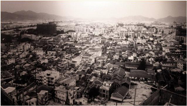
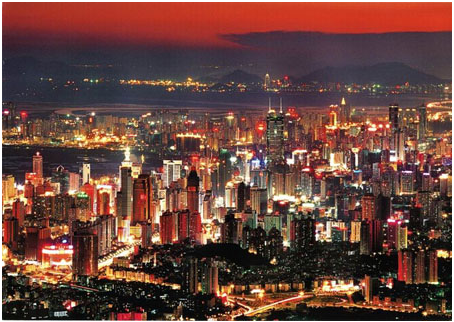
The Pearl River Delta, and particularly Shenzhen City, in Southern China has been going through a dramatic urbanization process since 1978 due to decentralization policies and market-oriented reforms.

Shenzhen City 1970

Shenzhen City 2011

%matplotlib inline
from IPython.display import IFrame
IFrame('http://svs.gsfc.nasa.gov/stories/Landsat/pearl_river.html','100%',490)

IFrame('https://earthengine.google.org/timelapse/player?c=https%3A%2F%2Fearthengine.google.org%2Ftimelapse%2Fdata&v=22.5500,114.1000,8.5&r=.5&p=true"','100%',490)

Shenzhen Plan of 2005

Purpose of the practical

In this project, we aim to quantify the change of land use due to urbanization, and attempt to explain such change by a number of important socioeconomical drivers. Yearly Landsat TM images are given from 1986 to present.

Overview of task

The project is most clearly phrased in two parts:

1. Classification of land cover from a series of Landsat images

As a first step, we need to quantify at least three types of land use for each given year, namely, urban, cropland, and other. In many circumstances, we would want to have cartegories of other as well, but this is not strictly necessary for this practical. Then, we can identify where changes have happened and how much land area has been transformed into urban. See example the land use change map below from Seto et al. 2002 as anexample of this.

We want to be able to classify quite a large number of images, so we need to bear that in mind when considering what approach to take.

A number of classification methods have been taught in this module, and Maximum Likelihood is often a good starting point for multispectral TM imagery. There are also other image processing methods could help to identify land use classes (e.g. vegetation indices, filters, segmentation, etc.). However, if we need to apply training for each scene, the task soon becomes very tedious. We could try to use the same training data for each scene, but this might not work well across multiple sensors.

Instead, we shall use a method of unsupervised classification (ISOdata clustering) to process the bulk of the data. This shifts the problem from one of large manual effort in providing the training datasets to a smaller manual effort making sure we interpret the machine-generated clusters appropriately. This is a basic trade-off of unsupervised versus supervised methods.

In this work then, you will apply a supervised method and an unsupervised method to one scene, then assess the classification accuracy of your approaches. Because of the large number of images involved in the project, we will use an envi program (provided to you) to automate the process of unsupervised classification for the rest of the datasets.

After you have performed the classifications, you will process each dataset to estimate the area of urban land cover per year. Again, because of the large number of images involved, we will use an envi program to do this.

2. Modelling Land Use change with socio-economic drivers

Having derived a dataset of urban land use, we can calculate urban land use change per year.

Following the general approach of Seto & Kaufmann (2003), we will build a multi-linear model to attempt to describe the urban land use change per year (the ‘y’ variable) as a function of a number of key socioeconomic factors (e.g. capital investment, land productivity, population, wage rates, etc) (the ‘\(x\)’ variables).

Following the example in the paper, we will use the following in \(x\):

• \(x_1\): Investment in capital construction / population
• \(x_2\): value of gross agricultural output / agriculture population
• \(x_3\): log(wages in non-state, non-collective units)
• \(x_4\): log(average total wage)
• \(x_5\): (value of gross agricultural output/Agricultural land) / (value of gross industrial output / Urban land)

This will give a model with 6 parameters that we need to estimate (i.e. 6 unknowns) that we could call \(p_0, p_1, p_2, p_3, p_4, p_5\). We could then write the model more specifically as:

Equation 1:

\[y = p_0 + p_1 x_1 + p_2 x_2 + + p_3 x_3 + p_4 x_4 + p_5 x_5\]

Note that the final term (\(x_5\)) requires that we have data for Agricultural and Urban land, which we will need to derive from the remote sensing data for each year of observation.

The rest of the data will come from official statistics.

Summary

The project involves the following tasks:

Data processing

• Download Landsat annual datasets for 1986 to present (or some suitable subset).
• For one year (your choice), perform a supervised classification and an unsupervised classification using envi and assess the accuracy of the classifications;
• Perform unsupervised classifications (clustering) of the time series of Landsat data, using an envi program that you will be provided with;
  • apply suitable class labels, and modify the number of classes as appropriate;
• Calculate the area of urban land use for Shenzhen for each year
• Estimate the area of agricultural land use for Shenzhen for each year (if possible, not critical)
• Try to assign a value of uncertainty to the derived data (from earlier accuracy assessment)

Modelling

Following the general approach of Seto & Kaufmann (2003), we will build a multi-linear model to attempt to describe the urban land use change per year (the ‘y’ variable) as a function of a number of key socioeconomic factors (e.g. capital investment, land productivity, population, wage rates, etc) (the ‘\(x\)’ variables).

Equation 1:

\[y = p_0 + p_1 x_1 + p_2 x_2 + + p_3 x_3 + p_4 x_4 + p_5 x_5\]

The model relates socio-economic variables (constant, plus x1, x2, x3, x4, x5), weighted by model parameters (p0, p1, p2, p3, p4, p5) to predict the rate if change of urban area per year (du_dy).

We have taken a set of observations of du_dy, derived from Landsat land cover classifications for the years 1986 to present (or a subset). Along with estimates of the x variables from the Guangdong yearbook, we have then seen how to produce an esrimate of the model parameters (the p terms).

Using the data derived above, calibrate a model that describes urban land use change as a function of a set of socioeconomic factors, following the approach of Seto et al. (2002, 2003). You are provided with R code and appropriate datasets to achieve this.

Analyse the statistics of the model and experiment to try to find an improved model with fewer parameters.

You are free to perform additional experiment, with the expectation of higher marks, provided (i) you have done the basic requirements well enough, and (ii) you show clarity of thoiught and understanding of what you are doing in your experiments.

Details

• Introduction
• ENVI Setup
• Modelling Setup
• Google Download
• Classification
• Modelling
• Project Write up
• Project Advice

Further Reading

Hao, P. (2012) Spatial evolution of urban villages in Shenzhen. PhD thesis University of Twente; Summaries in Dutch and English. ITC Dissertation 205, ISBN: 978-90-6266-295-1.

Seto, K.C., Woodcock, C.E., Song, C., Huand, X., Lu, J., and Kaufmann, R.K. (2002) Monitoring land-use change in the Pearl River Delta using Landsat TM, Int J. Rem. Sens, 23(10).

Seto, K.C., and Kaufmann, R.K., (2003) Modeling the Drivers of Urban Land Use Change in the Pearl River Delta, China: Integrating Remote Sensing with Socioeconomic Data, Land Economics, 79(1): 106-121

Using ENVI on your own computer

Introduction

In these notes, we outline how you can do the image processing coursework for GEOG0027 using remote access UCL computing resources in a browser on any computer Desktop@UCL Anywhere.

Desktop@UCL

First, make sure you have Desktop@UCL Anywhere setup and the relevant software installed. Just follow the instructions on Desktop@UCL Anywhere. If this has worked, you should see the following window in your browser:

Click on the Desktop icon to launch Desktop. This will give you a windows session, running in your browser, connected to your UCL account.

NOTICE ENVI is not currently installed on Desktop anywhere … Im getting that fixed … but for the moment use one of the other options

Stand-alone installation of ENVI

EVERY time you want to use this program you must be connected to the UCL domain (see below.

If you are using your own computer you will need to install the ENVI software and license from the UCL software database.

Downloading and Installing ENVI

Download ENVI from http://swdb.ucl.ac.uk/package/view/id/142?filter=envi, getting the appropriate version for your computer (Mac, Windows or Linux).

Follow the instructions on the screen to install the software.

Further instructions on how to install ENVI can be found here:

• Windows
• Mac

Once the installation has been completed you will be prompted to start the License Administrator select YES to begin the licensing process Select ‘User License Server’ and input lic-envi-idl.ucl.ac.uk as the server name and 7070 as the port number.

Click Connect and then close.

Set up a UCL VPN connection

If you are outside the university you will need to setup a Virtual Private Network (VPN) connection. This involves downloading software from ISD.

EVERY time you want to use this program you must be connected to the UCL domain.

For Windows:

• To setup a VPN connection please refer to https://www.ucl.ac.uk/isd/how-to/connecting-to-ucl-vpn-microsoft-windows

  

  This involves downloading, installing and running Cisco anyconnect software.

  Note that your machine needs to be running an anti-virus product. Further information on obtaining these products can be found at:

  http://swdb.ucl.ac.uk/?filter=firewall

  http://swdb.ucl.ac.uk/?filter=anti%20virus

Once installed, connect the VPN to vpn.ucl.ac.uk and follow the instructions below.

EVERY time you want to use ENVI you must be connected to the UCL domain.

For Mac:

• VPN

  To setup a VPN connection please refer to https://www.ucl.ac.uk/isd/how-to/connecting-to-ucl-vpn-mac-os-x

  This involves downloading, installing and running Cisco anyconnect software.

  Note that your machine needs to be running an anti-virus product. Further information on obtaining these products can be found at:

  http://swdb.ucl.ac.uk/?filter=firewall

  http://swdb.ucl.ac.uk/?filter=anti%20virus

• Additional software

  Note that, if you are using a Mac, you will need to install XQuartz as well (unless you already have it installed) to be able to use ENVI.

Once installed, connect the VPN to vpn.ucl.ac.uk and follow the instructions below.

EVERY time you want to use ENVI you must be connected to the UCL domain.

Using ENVI for GEOG0027

For Windows

Downloading the required files

• Create a folder on your device (e.g. on the Desktop) called GEOG0027. Within this, create a new folder called gee (standing for Google Earth Engine).

This is where you are going to do your work. You might, for instance, do this on your Desktop.

Note that the path of your working directory (that we will need later) will relate to how you set this up, so make a note of it now.

For example:

C:\Users\YOURUSERNAME\Desktop\GEOG0027\gee

• Go to the web page http://www2.geog.ucl.ac.uk/~plewis/GEOG0027/ and download the files:

  http://www2.geog.ucl.ac.uk/~plewis/GEOG0027/classy.zip

  http://www2.geog.ucl.ac.uk/~plewis/GEOG0027/gee.zip

• You may need some additional software to ‘unzip’ files. Some free software that works and UCL recommend is 7zip. Go to their website and install it (you will probably want the ‘64-bit’ version, unless you have a very old computer).

• When the data files (classy.zip and gee.zip) have downloaded (the gee.zip file will take a few minutes), you should just be able to click on them to run your software that will uncompress the files. You will want to extract them into your GEOG0027\gee folder:

]

You should now be able to navigate to your GEOG0027\gee folder and see the downloaded files:

1986 1987 1988 1989 1990 1991 1992 1993 1994 1995
1996 1997 1998 1999 2000 2001 2002 2003 2004 2005
2006 2007 2008 2009 2010 2011 2012 2013 2014 2015
2016 2017 2018 2019
classy.pro
classy_lut1.dat classy_lut3.dat classy_lut4.dat

Once you have successfully installed ENVI (above), navigate to C:\Program Files\HARRIS\ENVI and open ENVI + IDL (64 bit):

In the console that appears, type the following (adapted to where you have put your own data):

cd, ‘C:\Users\YOURUSERNAME\Desktop\GEOG0027\gee’

• The comma , and quotes ' are important!
• Don’t put YOURUSERNAME … put your username.

You will now be able to carry out the tasks we have been doing in the practical’s for example by loading the data into ENVI through this console which can then be opened in ENVI:

For Linux (Unix) or Mac

#### Command line and some unix commands

When, in the notes, we say ‘type at the command line’, we mean that youy should type the command in what you might call a Terminal or shelltool. On a Mac, find this under /Applications/Utilities/Terminal.app in Finder. On linux, it should be obvious (!).

The shell will show a prompt, e.g.:

%bash

To ‘type a command’, type at the prompt, then hit <return> to run the command.

% bash

It is helpful to know a few unix commands. The ones we will use are:

echo       :  print out a shell or environment variable
mkdir -p   :  create a directory (the -p option means not
              to complain if it already exists)
cd         :  change directory, i.e. move to somewhere on the
              file system.
pwd        :  print working directory
              (i.e. where am I in the file system?)
ls -lh     :  provide a listing of files. The -l option
              provides a 'long' listing. The -h option
              gives the file size in 'human readable' format

We need to make sure we are clear about where we will be working.

Let’s assume this is ${HOME}/DATA/GEOG0027/gee.

Try the following commands (don’t type the %%bash part):

%%bash

# print the value of ${HOME} (our home on the system)
echo "print a shell/environment variable value:"
echo ${HOME}
# the echo here is to print a blank line
# to space the text out. Not something you'd
# normally do!
echo

# create the data directory
echo "make a directory for our data"
mkdir -p ${HOME}/DATA/GEOG0027/gee
echo

# change to that directory
echo "Change directory to the data area"
cd ${HOME}/DATA/GEOG0027/gee
echo

# print where we are
echo "we are: (using pwd)"
pwd
echo

# see what files we have (this might be nothing at first!)
echo "get a long file listing"
ls -lh
echo

# sometimes, we will just use ls,
# a simple listing of what files there are:
echo "get a short file listing"
ls

print a shell/environment variable value:
/Users/plewis

make a directory for our data

Change directory to the data area

we are: (using pwd)
/Users/plewis/DATA/GEOG0027/gee

get a long file listing
total 6031232
drwx------  21 plewis  staff   672B  8 Feb 13:28 1986
drwx------  22 plewis  staff   704B  8 Feb 13:28 1987
drwx------  22 plewis  staff   704B  8 Feb 13:28 1988
drwx------  22 plewis  staff   704B  8 Feb 13:28 1989
drwx------  22 plewis  staff   704B  8 Feb 13:28 1990
drwx------  22 plewis  staff   704B  8 Feb 13:28 1991
drwx------  22 plewis  staff   704B  8 Feb 13:28 1992
drwx------  22 plewis  staff   704B  8 Feb 13:28 1993
drwx------  22 plewis  staff   704B  8 Feb 13:28 1994
drwx------  22 plewis  staff   704B  8 Feb 13:28 1995
drwx------  22 plewis  staff   704B  8 Feb 13:28 1996
drwx------  22 plewis  staff   704B  8 Feb 13:28 1997
drwx------  22 plewis  staff   704B  8 Feb 13:28 1998
drwx------  22 plewis  staff   704B  8 Feb 13:28 1999
drwx------  22 plewis  staff   704B  8 Feb 13:28 2000
drwx------  22 plewis  staff   704B  8 Feb 13:28 2001
drwx------  22 plewis  staff   704B  8 Feb 13:29 2002
drwx------  22 plewis  staff   704B  8 Feb 13:29 2003
drwx------  22 plewis  staff   704B  8 Feb 13:29 2004
drwx------  22 plewis  staff   704B  8 Feb 13:29 2005
drwx------  22 plewis  staff   704B  8 Feb 13:29 2006
drwx------  22 plewis  staff   704B  8 Feb 13:29 2007
drwx------  22 plewis  staff   704B  8 Feb 13:29 2008
drwx------  22 plewis  staff   704B  8 Feb 13:29 2009
drwx------  22 plewis  staff   704B  8 Feb 13:29 2010
drwx------  22 plewis  staff   704B  8 Feb 13:29 2011
drwx------  22 plewis  staff   704B  8 Feb 13:29 2012
drwx------  22 plewis  staff   704B  8 Feb 13:29 2013
drwx------  22 plewis  staff   704B  8 Feb 13:29 2014
drwx------  22 plewis  staff   704B  8 Feb 13:29 2015
drwx------  22 plewis  staff   704B  8 Feb 13:29 2016
drwx------  22 plewis  staff   704B  8 Feb 13:29 2017
drwx------  22 plewis  staff   704B  8 Feb 13:29 2018
drwx------  22 plewis  staff   704B  8 Feb 13:29 2019
-rw-r--r--   1 plewis  staff   6.4K  7 Feb 10:21 classy.pro
-rw-r--r--   1 plewis  staff   2.6K  8 Feb 13:21 classy.tar.Z
-rw-r--r--   1 plewis  staff   212B  7 Feb 02:09 classy_lut1.dat
-rw-r--r--   1 plewis  staff   119B  7 Feb 02:09 classy_lut3.dat
-rw-r--r--   1 plewis  staff   135B  7 Feb 02:09 classy_lut4.dat
-rw-r--r--   1 plewis  staff   2.9G  8 Feb 13:26 gee.tar.Z

get a short file listing
1986
1987
1988
1989
1990
1991
1992
1993
1994
1995
1996
1997
1998
1999
2000
2001
2002
2003
2004
2005
2006
2007
2008
2009
2010
2011
2012
2013
2014
2015
2016
2017
2018
2019
classy.pro
classy.tar.Z
classy_lut1.dat
classy_lut3.dat
classy_lut4.dat
gee.tar.Z

Pull some files from the internet

We will now pull some data and code files we need for this work. They are all available through the link http://www2.geog.ucl.ac.uk/~plewis/GEOG0027, but we can directly pull the files from the command line.

To do this, we need two more unix commands:

curl       :  get a file from a URL
tar        :  File comnpression and uncompression

Pulling the files will take a little time, but you only need to do this once!

%%bash

# just to be safe, make sure we have the data directory!
mkdir -p ${HOME}/DATA/GEOG0027/gee
# and go there
cd ${HOME}/DATA/GEOG0027/gee

# pull the code file:
curl http://www2.geog.ucl.ac.uk/~plewis/GEOG0027/classy.tar.Z -o classy.tar.Z
# pull the data file: this will take a few minutes!!
curl http://www2.geog.ucl.ac.uk/~plewis/GEOG0027/gee.tar.Z -o gee.tar.Z

  % Total    % Received % Xferd  Average Speed   Time    Time     Time  Current
                                 Dload  Upload   Total   Spent    Left  Speed
100  2622  100  2622    0     0   102k      0 --:--:-- --:--:-- --:--:--  102k
  % Total    % Received % Xferd  Average Speed   Time    Time     Time  Current
                                 Dload  Upload   Total   Spent    Left  Speed
100 2944M  100 2944M    0     0  10.4M      0  0:04:41  0:04:41 --:--:-- 11.2M

This should have pulled the files we need to the local file system.

We can check this, and then uncompress the files:

%%bash

# just to be safe, make sure we have the data directory!
mkdir -p ${HOME}/DATA/GEOG0027/gee
# and go there
cd ${HOME}/DATA/GEOG0027/gee

# get a long listing of the pulled files
# to see they are the right size
ls -lh classy.tar.Z gee.tar.Z

# uncompress them
tar xvzf classy.tar.Z
tar xzf gee.tar.Z

-rw-r--r--  1 plewis  staff   2.6K  8 Feb 13:21 classy.tar.Z
-rw-r--r--  1 plewis  staff   2.9G  8 Feb 13:26 gee.tar.Z

x classy_lut1.dat
x classy_lut3.dat
x classy_lut4.dat
x classy.pro

Let’s just do a final check that the files are there:

%%bash
cd ${HOME}/DATA/GEOG0027/gee

# now ls
ls

1986
1987
1988
1989
1990
1991
1992
1993
1994
1995
1996
1997
1998
1999
2000
2001
2002
2003
2004
2005
2006
2007
2008
2009
2010
2011
2012
2013
2014
2015
2016
2017
2018
2019
classy.pro
classy.tar.Z
classy_lut1.dat
classy_lut3.dat
classy_lut4.dat
gee.tar.Z

Using ENVI

Now we have the files and setup we need, we can simply run envi. To do this, type envi at the command line prompt:

%%bash
/Applications/harris/envi/bin/envi

IDL 8.7.0 (darwin x86_64 m64).
(c) 2018, Harris Geospatial Solutions, Inc.

Licensed for use by: University College London-CHEST
License: 405435-CHEST:****-****-****-B2C6
License expires  5-Mar-2019.
A new version is available: IDL 8.7.1
https://harrisgeospatial.flexnetoperations.com

% Restored file: ENVI.
% Loaded DLM: PNG.
% Loaded DLM: HPGRAPHICS.
% Loaded DLM: XML.

Summary

In this section, we have learned how to install the data files and software needed to do the coursework on your own computer, for your convenience. You can use all of the (linux) machines in the Geography lab, as we do in class, without the need for your own computer or any of this installation. Ideally, this should all be available on Desktop@UCL but that is not currently the case.

• Instructions summary / checklist:
  • Download and install ENVI and active license
  • Set up and install VPN
  • Windows: Download the data files and run ENVI + IDL
  • Mac or Linux: Download the data files and run envi

Install software and files for modelling

Setup options

Using R or Rstudio

There are several ways you can develop and run the modelling code we will be using.

We will be using the R software that you should be familiar with for the first year. If you need to refresh you memory with what you did in GEOG0013, we provide the relevant files for you on moodle. Try to make sure you are familiar with loading csv files, basic graphing, and performing linear regression.

Which option should I choose?

It is probably easiest for you to use the RStudio environment for this work. First, this should be what you are familiar with. Second, it is convenient to use to develop codes and save the results as a report. Third, it is much easier to use with these notes.

On the UCL Geography computers, we don’t have Rstudio, only R. You should be able to use this, but it doesn’t give you the fancy interface.

The options for software environments for doing this part of the work are:

1. Run R on the Geography UCL (Linux) computers
2. Run Rstudio using Windows on Desktop@UCL Anywhere
3. Run Rstudio (or R) on your own computer
4. Run Rstudio on binder
5. Run R (via Python) on Jupyter

The advantage of using option 1. is that you don’t need to do anything other than come along and use the computers in the Geography Unix lab. Whilst there are ways you can access this remotely, it is perhaps not the easiest thing for you to do so, so if you intend working outside of the lab a lot, then consider another option. Also, you don’t have access to RStudio in this option.

Options 2-4 would probably be the best for you to consider.

Option 5 is very neat, and involves running the codes in a notebook (this is a notebook you are using now!). But it is more complex to explain how to do this. If you are particularly interested in this sort of computing, we will help individuals to go through this route on request.

Option 3 needs you to set up software. Options 2 and 3 need you to install data and code files.

Option 4 has everything set up for you, runs in any browser (so, even on your phone or tablet), on an external server, but you are at risk of losing your work if you let the session go idle for 10 minutes or more, or if your session lasts longer than 12 hours. You can of course save and reload your work, but you have to be more careful of this in option 4. Also, option 4 takes a few minutes to get started, as it has to run a remote server.

Installing R and Rstudio on your own computer

Option 3 involves setting up R and Rstudio on your own computer.

To install the packages you need for R and RStudio, follow the links below to download and install the software. Check it works by starting RStudio.

• Download and install R from https://cran.rstudio.com
• Download and install RStudio from https://www.rstudio.com

Installing data packages

Best way (recommended)

A preferable way to do this, is to access these notes directly from RStudio.

Once you have started RStudio on any computer, start a new project:

Then select Version control:

Then git:

Fill in the form, with:

Repository URL as https://github.com/profLewis/GEOG0027_Coursework.git

Project directory name as some suitable name you will remember

and

Create project as subdirectory of: somewhere suitable, e.g. Desktop/GEOG0013

This will then download the GEOG0027_Coursework git repository. This has the advantage of containing all of the codes, files and notes.

After you have installed this, you should be able to navigate to the GEOG0027_Coursework/docs/files folder, and click on the icon for GEOG0027_Coursework.Rproj to start the RStudio session.

Minimal way (not recommended)

For options 2 and 3, the minimal data/code requirement is that you install a few data and software packages. This involves downloading the file UrbanModel.zip and unzipping and storing it in your workspace (e.g. in GEOG0027/gee).

Option 1

In a terminal (shelltool), change directory to where your data files are.

Start R by typing R at the command line prompt.

Follow the instructions in the Modelling section, typing R commands at the R prompt.

Option 2

Start Desktop@UCL Anywhere in a browser.

Start RStudio, and run RStudio as directed above.

Option 3

Install R and Rstudio.

Start RStudio on your computer, and run RStudio as directed above.

Option 4

Start RStudio by clicking the binder badge, and run RStudio as directed above:

Then:

1. Upload any previous session files.

This will create a folder called (e.g.) rstudio-export.

We need to restore the files from here to the working directory.

To do this:

• in the Files panel, click on the folder you have just uploaded (rstudio-export) to ‘go into’ that folder.
• Select all of the files you want to move (tick the check boxes):

• and move the files to the normal working folder:

Note that this will over-write the files in that folder.

• finally, delete the (now empty) rstudio-export folder

2. Do your work in RStudio as usual
3. Save and download your session files.

To do this:

• select the files you want to save (check boxes)
• Under the More menu, select Export ...

• and save the file (rstudio-export.zip) to your local file system.

You can use this same approach to transfer files between any different RStudio sessions you are running on different computers.

Option 5

One way to use option 5 is to start this page in Binder:

Running Rstudio

Select the .Rproj file

There should be an file that ends .Rproj in your folder docs/files

If you click on this, then RStudio should load up, with information from any previous sessions.

Alternatively, start RStudio any other way.

Set working directory

In RStudio, check to see where your files panel (bottom right) is showig. If this isn’t your data area, navigate to where your data and code files are, and set this as the working directory.

You will need the following files, so check they exist in your data folder!

Required files

Guandong-Yearbook-2019.csv

model-2019.csv

results-2019.csv

UrbanModelData.R

UrbanModel.R

Load and run UrbanModelData.R

Select the file UrbanModelData.R so that it appears in the code window:

Then run the source file (this will run UrbanModelData.R)

Now we’ve seen that it works, you can look through the code in a little more detail.

This code loads the datasets you need, runs a linear regression, and plots appropriate graphs. We will go through this in detail in the modelling section, but you should try to understand the basic layout and operation of the codes.

Save the R file regularly

When working, you will be able to save the R file after you have made any edits. Make sure you do so quite regularly. You may like to check the source on save tick box, which then re-runs your script when you save it (to see you haven’t broken it)

Binder care

If you are using the binder interface, then before you quit any session (and perhaps from time to time in a session), make sure you save any files you might need, and download them to the local computer (to store somewhere safe).

To do this:

• select the files you want to save (check boxes)
• Under the More menu, select Export ...

• and save the file (rstudio-export.zip) to your local file system.

You can use this same approach to transfer files between any different RStudio sessions you are running on different computers.

If you quit RStudio, you should be asked whether you want to save the workspace. Do so, so then the next session (next time you run RStudio) you can start where you left off.

Write a report

Once you have done some work (in the modelling section) you will want to save the R file (above) but you may also want to generate a report on your script. One good way to do this is to save the report as a Word file (assuming you have MS Word installed on your computer).

To do this, click on the compile report button:

Change the report format to MS Word and compile the report.

The file, a formatted version of your code and output such as graphs, will be saved into the local directory UrbanModelData.docx. You will find these useful when you come to write your reports. Dont however

Download and visualise data

Download

In this section, you will learn how to download data using a web-based app developed using Google Earth Engine (GEE). GEE has access to a large number of Earth Observation and other datasets, and makes it easy to access these and do a some processing (at least for a limited spatial extent if you want high resolution data).

You are provided with a web App built using GEE:

This is available to you as a specific App for the Shenzhen area. The use of the App should be quite intuitive, but we will outline how to use it below.

The app gives you access to 5 bands of Landsat surface reflectance data (see figure below), along with two vegetation indices, NDVI and NDWI. The datasets are annual composites, with each pixel the median of valid surface reflectance data for that year.

First load the App:

%matplotlib inline
from IPython.display import IFrame
IFrame('https://plewis.users.earthengine.app/view/shenzhen','100%',490)

By default, a composite dataset for the year 1986 is loaded, along with a rough initial classification.

You can download these datasets from this interface by clicking on:

• the 1986 link to get the Landsat composite dataset
• the header link to get the associated envi header files

You should download these files and unzip them into an appropriate directory in your Data directory (e.g. ~/Data/GEOG0027/1986). You can also access the classification files class but there is little point downloading these as we will not use them.

You can change the year of the dataset in the right-hand panel. You can also load data for multiple years, although the App response may become slow (depending on network speeds). You can clear the loaded datasets with the Clear ... button.

For example (N.B. once you have downloaded the files):

%%bash

# where the zip files are now, *after* having downloaded them
in=./files
# where we will put the files
out=~/DATA/GEOG0027/

mkdir -p $out
unzip -u $in/1986.zip -d $out
unzip -u $in/1986_hdr.zip -d $out
mv $out/class1986/* $out

You may find it more straightforward to use any tool prompted by your browser when downloading and extracting these files. In any case, make sure that all files for all archives go into a folder that is named after the year of the dataset (1986 here). This is important for automatic further processing later.

Getting the data archive

Whilst you should find it instructive to download the datasets from the App, it is a little tedious to do that for all of the datasets.

For this reason, on the UCL Geography system, you can access the entire dataset from a single file.

To use this, open a Unix shell, and type the following:

%%bash

data=/home/plewis/public_html/GEOG0027/gee.tar.Z
out=~/DATA/GEOG0027/

mkdir -p $out
cd $out
tar xzf $data

If you are outside the UCL Geography system, you can access the archive file as a compressed tar archive from either of these links [tar file or zip file], but beware that the compressed file is 2.9G.

Visualise time series

You may have noticed a time series graph on the left-hand panel of the app. This appears when you click on any location in the image panel, and provides a visualisation of the time series of reflectance (and vegetation indices) for that location. You can pop the graph out to another browser tab (the grey square with arrow in the top left of the plot).

It will look like this:

This is useful foir giving you an idea of the land cover history of this location, so you might want to produce graphs for several locations with different cover types, to use in your report.

You can directly save the plot (Download png button) or save the dataset (Download csv button).

If you download the csv file, you can then produce your own plots of the data (for your report).

The example below are given in Python, but you should use whatever graphing package you are familiar with. Please make sure that (unlike below, which are for illustration only) you put full titles, labels and legends on graphs.

import matplotlib.pylab as plt
%matplotlib notebook
import numpy as np
import pandas as pd

d = pd.read_csv('files/ee-chart.csv')
d

	system:time_start	B1_blue	B2_green	B3_red	B4_nir	B5_swir	B6_NDVI	B7_NDWI
0	1986-06-06	0.102	0.175	0.238	0.347	0.388	0.187	-0.055
1	1987-06-06	0.103	0.177	0.227	0.299	0.412	0.136	-0.159
2	1988-06-06	0.101	0.157	0.206	0.296	0.315	0.181	-0.030
3	1989-06-06	0.104	0.158	0.192	0.262	0.295	0.154	-0.058
4	1990-06-06	0.154	0.221	0.272	0.330	0.381	0.097	-0.072
5	1991-06-06	0.133	0.187	0.211	0.260	0.300	0.105	-0.072
6	1992-06-06	0.145	0.185	0.205	0.239	0.295	0.078	-0.104
7	1993-06-06	0.144	0.188	0.205	0.249	0.293	0.098	-0.081
8	1994-06-06	0.111	0.139	0.149	0.181	0.227	0.098	-0.114
9	1995-06-06	0.114	0.136	0.137	0.170	0.213	0.109	-0.111
10	1996-06-06	0.107	0.132	0.137	0.159	0.192	0.074	-0.095
11	1997-06-06	0.098	0.121	0.132	0.162	0.190	0.104	-0.079
12	1998-06-06	0.125	0.150	0.160	0.183	0.215	0.064	-0.081
13	1999-06-06	0.123	0.152	0.167	0.183	0.200	0.045	-0.045
14	2000-06-06	0.134	0.153	0.157	0.167	0.203	0.031	-0.096
15	2001-06-06	0.110	0.131	0.140	0.152	0.166	0.038	-0.045
16	2002-06-06	0.115	0.132	0.134	0.146	0.138	0.041	0.027
17	2003-06-06	0.113	0.128	0.138	0.153	0.152	0.054	0.004
18	2004-06-06	0.133	0.169	0.186	0.218	0.257	0.079	-0.082
19	2005-06-06	0.140	0.181	0.199	0.233	0.257	0.079	-0.050
20	2006-06-06	0.141	0.171	0.178	0.221	0.226	0.106	-0.012
21	2007-06-06	0.141	0.186	0.205	0.242	0.257	0.084	-0.029
22	2008-06-06	0.154	0.183	0.186	0.235	0.232	0.117	0.007
23	2009-06-06	0.145	0.170	0.180	0.211	0.217	0.078	-0.014
24	2010-06-06	0.151	0.180	0.184	0.213	0.228	0.073	-0.035
25	2011-06-06	0.144	0.169	0.175	0.202	0.227	0.072	-0.059
26	2012-06-06	0.144	0.169	0.175	0.202	0.227	0.072	-0.059
27	2013-06-06	0.127	0.156	0.165	0.216	0.215	0.135	0.003
28	2014-06-06	0.114	0.145	0.155	0.202	0.197	0.131	0.013
29	2015-06-06	0.128	0.158	0.169	0.226	0.240	0.144	-0.029
30	2016-06-06	0.117	0.146	0.157	0.221	0.240	0.168	-0.040
31	2017-06-06	0.123	0.153	0.161	0.209	0.209	0.129	0.001
32	2018-06-06	0.140	0.176	0.188	0.242	0.253	0.125	-0.023

Note that the time label for each dataset is YYYY-06-06. The day and month (06-06) have no significance here as this is an annual composite dataset.

_=d.plot(figsize=(10,4),title='Example data plot')

Visualise spatial data

You should be able to conveniently explore the spatial datasets in the GEE App. This is particularly useful for data interpretation (e.g. for training or validation) as you can have a map or high resolution image as a background.

You can also load multiple years of data, and visualise the dynamics.

Other than that, you will probably want to load the datasets into envi for visualisation. If you have correctly stored the data from the zip files, you should have in your data directory a series of sub-directories named by year, such as:

1986    1989    1992    1995    1998    2001    2004    2007    2010    2013    2016    2019
1987    1990    1993    1996    1999    2002    2005    2008    2011    2014    2017
1988    1991    1994    1997    2000    2003    2006    2009    2012    2015    2018

Inside each of these, you should see files such as the following:

22014.constant.tif     2014.swir.tif
2014.NDVI.tfw           2014.green.tfw
2014.NDVI.tif           2014.green.tif
2014.NDWI.tfw           2014.nir.tfw
2014.NDWI.tif           2014.nir.tif
2014.blue.tfw           2014.red.tfw
2014.blue.tif           2014.red.tif
2014.constant.tfw       2014.swir.tfw
2014_Shenzhen            2014_Shenzhen.hdr

The file 2014_Shenzhen is particularly important, as this is the file that you will load using envi.

One further file that may be of interest is the file 2014.constant.tif which you can use as a data mask if you like. The mask has a value of zero for Shenzhen and no data outside of that.

You should load and explore the datasets you have downloaded. Provide examples of e.g. interesting spectral profiles, transects, histograms or scatter plots for your report – things that you would normally produce as part of a data exploration exercise.

the histograms are of interest (think about what this means for classification)

and the scatterplots in many ways even more interesting:

You will find it particularly interesting to examine scatter plots of NDVI and NDWI for this dataset as you should see that a pretty good classification can be achieved with just these two bands of data. An advantage of this would be that the processing should be faster (fewer bands), but also that it is straightforward to visualise and appreciate the clusters that will be used to describe the land cover classes.

These are not the only ‘bands’ to explore though! Collect plenty of images of scatterplotas, histograms and images for your write up to illustrate particular things you find. Don’t just put images in the report with no reference to what you are using them to show!

You should spend some time exploring these scatterplots for the different years data: are the patterns consistent? (show some evidence). Can you simply visualise (and explain) the clusters and their relationship to land cover types? In exploring the datasets you should save interesting plots to use in your write-up – anything that helps you explain what is going on is of value!

ENVI Classification

Data processing summary of requirements

[60% of marks in total Classification]

Data Exploration and Classification Theory

[30% of marks]

Select data for a single year and download from Google Earth Engine App supplied

For the data selected for the single year:

• Choose one supervised and one unsupervised classification approach (we recommend Maximum Likelihood and ISOData
• Theory: describe how the approaches work (noting similarities and differences) and relate this to the information content of your data. Cite literature as appropriate. [10%]
• Perform a supervised classification and an unsupervised classification using envi, relating the training information (e.g. class seperability) to the material presented above;
• Present the results of the classification and assess the accuracy of these classifications; [15%]
• Discuss the issues raised and how this might translate to unsupervised classification of the whole time series. [5%]

Time Series Classification

[30% of marks in Part 2b]

• Download Landsat annual datasets for 1986 to present (or some suitable subset of at least 18 years): you can copy the data from the GEOG0027 archive
• Perform an unsupervised classifications (clustering) of the time series of Landsat data, using an envi program that you will be provided with (classy.pro);
• apply suitable class labels, and modify the number of classes as appropriate;
• Calculate the area of urban land use for Shenzhen for each year
• Estimate the area of agricultural land use for Shenzhen for each year (if possible, not critical)
• Try to assign a value of uncertainty to the derived data (from earlier accuracy assessment)
• Write up this section of work, describing:
  • the tasks undertaken (materials and method) [5%]
  • the experiments conducted (e.g. with varying class number/waveband) [10%]
  • the results and uncertainty [10%]
  • discussion of the results (in context of text above) [5%]

Prepared by:

Dr Qingling Wu, Prof Philip Lewis, Dr Mathias Disney

Contact: Professor Lewis

---

Extraction of land use extent

Your task in this section is to calculate the area of land cover & land use (LULC) extent (in \(m^2\)) for each year of a series of Landsat imagery. If possible, you should provide an associated characterization of uncertainty in each of these areas.

Along the way, you will need to do a manual classification (one supervised, one unsupervised) in envi. As a first step, we should try to quantify at least three types (urban, agricultural, and other) of land uses for each given year. A number of classification methods have been taught in this module, and Maximum Likelihood is a good starting point for multispectral TM imagery. There are also other image processing methods could help to identify land use classes (e.g. vegetation indices, filters, segmentation, etc.). Then, we can identify where changes have happened and how much land area has been transformed into urban built.

You then need to run an automated processing script classy.pro in envi to apply unsupervised classification to the whole time series of data.

For the modelling section of this report, it is critical that you extract a reasonable estimate of urban land cover for each year (it is not vital to do every year, but once you get started, this should not be too much bother). Agricultural land use should only be attempted if it proves feasible. If you do not believe it so, make a case in your report for not generating this cover class, and make sure you provide evidence to back this up. An acceptable excuse might,, for instance be that agriculture cannot be easily distinguished from other vegetation types in an annual dataset, but you would need to provide evidence of this. Also, some of the agricultural land use in the region is rice paddies, which might have rather similar signatures to other shallow water areas (if you want to claim that, provide evidence, e.g. spectra).

Obtaining Landsat data

See the section Google Download for information on how to obtain and explore data. You should go through this section carefully, building your understanding of the datasets you are using. Take note of the ‘hints’ as to what might be interesting to explore (and put in your report). We suggest you access data using this approach.

An alternative source of data is direct from the USGS, which you can explore in the Download page, including how to search only for the area we are interested in. It is certainly not critical that you explore this for this practical, but you should find it of general use, and might, for example, use it to discuss issues (e.g. cloud) with using individual Landsat scenes, rather than the composites we make available via Google Earth Engine.

In any case, remember to write up each of the steps you go through in producing the input dataset for classification, and provide appropriate evidence. Note the guidelines and weightings given at the top of this section.

Classifying the data: manual method

You should now have a set of (annual) image subsets (and associated masks, if required) of the area of interest.

You next need to generalise the datasets into classification maps.

Although we will process the bulk of the data automatically, you will need to show that you can do a ‘manual’ classification.

For this reason, we require you to select one year (your choice) and perform a supervised classification and an unsupervised classification using ``envi``.

You should provide an assessment of the accuracy of the classifications (truth tables), concentrating on the ability to distinguish urban, agriculture and other (you may go into more detail with other).

You can use these accuracy assessments as an estimate of the uncertainty in the classifications when it comes to the modelling section (e.g. if you get an 80% accuracy on the urban class, you could suggest that there is roughly a 20% error on this class).

You can either work on the whole extent of the downloaded dataset, or just use a mask for the Shenzhen region. Make sure you are clear about which of these you have chosen to do.

Automated processing

We will use an ISOData clustering approach to process the full time series of data. You should make sure you are familiar with this approach and any issues in its use. As it is an unsupervised method, you will need to specify the number of classes you want. This choice should be based (at least initially) on your assessment of the datasets (e.g. the clusters you see in the NDVI / NDWI scatterplots):

Note that the automated processing will use only the NDVI and NDWI channels of information (‘bands’ if you like), by default for ease of processing and interpretation. You do have control over which bands are used, so you should experiment with that (e.g. cluster using all bands, or just vegetation indices).

Note that your results will be over-written each time you run the ``envi`` scripts so you will want to make copies of results for a particular setting (e.g. bands. or number of clusters)

To use the automated processing, you should first download the relevant files and place them in your data directory.

Loading the automation software

Start envi.

You should have a window (terminal/shell) that shows the ENVI> prompt. This is where we will type ’envi(actually,IDL`) commands.

First, make sure you are in your data directory:

ENVI> CD, '~/DATA/GEOG0027'

You can type Unix commands at this prompt if you put a $ before the command, so if we want to check the files that are there, type:

ENVI> $ls

You should see the following:

1986        1994        2002        2010        2018
1987        1995        2003        2011        2019
1988        1996        2004        2012        classy.pro
1989        1997        2005        2013        classy_lut1.dat
1990        1998        2006        2014
1991        1999        2007        2015
1992        2000        2008        2016
1993        2001        2009        2017

The automation code is in the file classy.pro, so we will get envi to load this:

ENVI> .compile classy

This should respond with:

% Compiled module: REAL_CLASSY.
% Compiled module: CLASSY.
% Compiled module: FIX_CLASS.
% Compiled module: MAKE_GIF.
% Compiled module: MAKE_MOVIE.

which is a list of the modules available to you.

We can explore first CLASSY.

; NAME:
;   classy
;
; PURPOSE:
;   Performs classification (clustering) on image
;   using ISOdata
;
; INPUTS:
;   input_file - name of envi image to read
;   nclasses - how many classesa (default 5)
;   bands    - band numbers to use (default [5,6])
;              use 0 for the 1st band. Max of 6
;
; OUTPUTS:
;    input_file + '_class'   - classification ENVI file
;
; AUTHOR:
;   P.Lewis, UCL 26 Jan 2019 (p.lewis@ucl.ac.uk)
;

Let’s first look at a Landsat file '2000/2000_Shenzhen. We can load this into envi and visualise the Vegetation indices:

We can see from this (and the scatter plot) that these two bands alone provide a good deal of discrimination of the main cover types. Let’s have a go at generating 3 clusters:

For this module, you specify an input_file to process, and optionally the number of classes and the image bands to use (specify as e.g. [0,1,2,3,4,5,6] for all bands), so, for example:

ENVI> CLASSY, '2000/2000_Shenzhen', 3, [5,6]

The result of running this should be an envi file 2000/2000_Shenzhen_class.

You can load that into envi using the usual menu system:

and we can see that this has been quite effective at pulling out 3 main cover types, namely water (Class 1 in red), bare soil and urban (Class 2 in green) and vegetation (Class 3 in blue). You should refer back to the original RGB image to confirm these interpretations:

You might decide that 3 clusters is sufficient: we have a vegetation class, even if its not explicitly agriculture, and we have an urban class (even though it probably includes areas of bare land as well).

If we decide that this is enough, we can process the whole time series on this basis.

First, we need to generate a text file to translate the class labels and colour to something more convenient.

We use a look up table (LUT) text file classy_lut3.dat:

Unclassified, 0,   0,   0
Water, 0,   0,   255
Urban, 200,   30, 0
Vegetation, 20, 200, 0
Masked Pixels, 64,  64,  64

This has, as well as the 3 clusters we wanted, a specification for Unclassified (class label 0) and Masked Pixels (class label 4) in case there are either of these.

Other than that, each line gives comma separated values of:

NAME, R, G, B

where NAME is the class name we want to use, and RGB are numbers between 0 and 255 that specify the colour and intensity to use. For example 0, 255, 0 would be bright green, 255, 255, 0 would be bright yellow.

Lets use this now to re-code the dataset:

ENVI> FIX_CLASS,'2000/2000_Shenzhen','classy_lut3.dat'

where we specify the file to operate on, and the LUT file.

This results in:

which is an appropriate interpretation of the clusters.

Note that if you change the wavebands used or the number of clusters, your image result will be over-written. To avoid this, open the dataset in envi, and save with a different filename (eg one containing the bands used and number of classes)

Of course, we might decide to use more clusters (7 here) to get more subtle interpretations, but we will find the classes rather harder to interpret. Possibly the best answer lies somewhere in between. You will need to explore that and come to some (justified) conclusion.

Once we decide that we have probably got a good set up (and an appropriate LUT file), we can set the whole time series processing:

ENVI> REAL_CLASSY,'.','classy_lut3.dat',[5,6]

This uses the module REAL_CLASSY and then specifies the directory to work in (. is the current directory, which is appropriate here), and then the LUT file to use, and the bands as above (use [0,1,2,3,4,5,6] for all bands). The number of classes to use is inferred from the number of entries in the LUT file.

This script will take a few minutes (or a little longer if more classes are specified), but will look over all of the directories containing the annual Landsat datasets (specified by year).

Once this is done, it applies the specified LUT to the classifications, and then generates a series of gif files that you can use in your report (each with the year labelled on the classification image).

Finally, an animated gif ‘movie’ is created:

You should use this animation (and the associated gif files) to come to some conclusions about your selection of the number of classes. In this case, we can see that the Water class is useful and stable (although it includes rice paddies in the top left of the image). There seems to be some jumping around between the vegetation and urban classes however: we would generally expect an increase in the urban area and a decrease in the vegetation over time. Because we have only used 3 classes here, the clusters that form sometime include other features, such as bare land, and sometimes don’t. This means that our class efinitions aren’t very stable.

It may be that some subset of the years that we have processed appears stable, and that may be enough to perform the modelling: in essence, we need at least 6 years of data over the time period for which we have the socioeconomic data to be able to provide an estimate of the 6 model parameters. Ideally, we should have at least twice that number.

If not, you may wish to explore other numbers of clusters and the wavebands used. Make sure you note down your experimentation (with plenty of appropriate figures) in your report. Make sure you save each classified image set you derive if you change the bands or n umber of clusters.

Pixel counting

Finally, you will need to provide a count of the total area of each class, with each pixel being 30 m x 30 m. To do this, you need to count how many pixels are in each class.

You can do this in envi following the menu items (right hand panel) Classification -> Post Classification -> Class Statistics.

This will produce the data you need to track land cover for each date. Make a note of the pixel counts for each year.

Alternatively, the module getstats (in classy.pro):

getStats,fixfile,results

will write the pixel counts, with appropriate headers, to a CSV format file results-YEAR.csv, where YEAR is the year you perform the experiment (so, 2019 in 2019).

An example output is:

Year,Unclassified,Water,Urban,Soil,Vegetation,Masked Pixels,
1986 ,           0 ,     1688763 ,      728147 ,     1599277 ,     1605031 ,           2 ,
1987 ,           0 ,     1686052 ,      966379 ,     1422736 ,     1546047 ,           6 ,
1988 ,           0 ,     1688295 ,      753086 ,     1554130 ,     1625708 ,           1 ,
1989 ,           0 ,     1698172 ,      664438 ,     1599387 ,     1659223 ,           0 ,
1990 ,           0 ,     1676593 ,      622059 ,     1592331 ,     1730237 ,           0 ,
1991 ,           0 ,     1692487 ,      678761 ,     1492200 ,     1757772 ,           0 ,
1992 ,           0 ,     1714083 ,      836708 ,     1531097 ,     1539332 ,           0 ,
1993 ,           0 ,     1703089 ,     1033756 ,     1377726 ,     1506649 ,           0 ,
1994 ,           0 ,     1690201 ,     1077816 ,     1355426 ,     1497777 ,           0 ,
1995 ,           0 ,     1663186 ,     1114267 ,     1440417 ,     1403216 ,         134 ,
1996 ,           0 ,     1657710 ,     1127971 ,     1437053 ,     1398486 ,           0 ,
1997 ,           0 ,     1660290 ,     1078099 ,     1450867 ,     1431964 ,           0 ,
1998 ,           0 ,     1635837 ,     1087832 ,     1375363 ,     1522183 ,           5 ,
1999 ,           0 ,     1637807 ,     1221455 ,     1436375 ,     1325578 ,           5 ,
2000 ,           0 ,     1650428 ,     1160521 ,     1331673 ,     1478591 ,           7 ,
2001 ,           0 ,     1625689 ,     1172997 ,     1387558 ,     1434976 ,           0 ,
2002 ,           0 ,     1611018 ,     1234615 ,     1413538 ,     1362048 ,           1 ,
2003 ,           0 ,     1597141 ,     1295468 ,     1290879 ,     1437730 ,           2 ,
2004 ,           0 ,     1580141 ,     1386381 ,     1287383 ,     1367297 ,          18 ,

Summary

[60% of marks in total Classification]

Part 2a: Data Exploration and Classification Theory

[30% of marks in Part 2a]

For the data selected for the single year:

• Choose one supervised and one unsupervised classification approach (we recommend Maximum Likelihood and ISOData
• Theory: describe how the approaches work (noting similarities and differences) and relate this to the information content of your data. Cite literature as appropriate. [10%]
• Perform a supervised classification and an unsupervised classification using envi, relating the training information (e.g. class seperability) to the material presented above;
• Present the results of the classification and assess the accuracy of these classifications; [15%]
• Discuss the issues raised and how this might translate to unsupervised classification of the whole time series. [5%]

Part 2a: Time Series Classification

[30% of marks in Part 2b]

• Download Landsat annual datasets for 1986 to present (or some suitable subset of at least 18 years): you can copy the data from the GEOG0027 archive
• Perform an unsupervised classifications (clustering) of the time series of Landsat data, using an envi program that you will be provided with (classy.pro);
• apply suitable class labels, and modify the number of classes as appropriate;
• Calculate the area of urban land use for Shenzhen for each year
• Estimate the area of agricultural land use for Shenzhen for each year (if possible, not critical)
• Try to assign a value of uncertainty to the derived data (from earlier accuracy assessment)
• Write up this section of work, describing:
  • the tasks undertaken (materials and method) [5%]
  • the experiments conducted (e.g. with varying class number/waveband) [10%]
  • the results and uncertainty [10%]
  • discussion of the results (in context of text above) [5%]

Project Write up

Assessment

• 100% Assessed Practical (3500 words) - submission date: Friday 22th March 2019 (12 noon) via moodle.

NB:

• Penalties for late submission and over length WILL be applied
• Different arrangements for JYA/Socrates (make sure you inform the lecturers if this affects you)

Requirements

A reminder of the project requirements. This is repeated from text given at the appropriate sections in the notes. Note the marking guidelines to give you an idea of how much effort to put into each part.

Part 1: Introduction (20%)

[20% of marks in total for Part 1]

Provide an introduction to the the purpose of the study: [5%]

• briefly covering why we might want to monitor and model urban change (and urban change in Shenzhen, in particular). Outline previous studies.
• Outline what is to be done in the rest of the study. Cite literature as appropriate.

For one year (your choice between 1986 and last year , but state the year used):

• describe a method of manual data download (e.g. using the Google Earth Engine App), with illustrations as appropriate. Note any processing that has been already done to the dataset, and which wavebands are made available to you, with equations as appropriate. [5%]
• Explore the dataset (histograms, scatterplots) to assess its information content (use figures); [10%]

Part 2: Data processing (60%)

[60% of marks in total for Part 2]

You must include an accuracy assessment for each manual classification you perform (so, for just one year).

The section or sub-section should contain ‘full-sized’ (on the page) pictures of the manual classification results, along with an appropriate table to interpret the colours.

Part 2a: Data Exploration and Classification Theory

[30% of marks in Part 2a]

For the data selected for the single year:

• Choose one supervised and one unsupervised classification approach (we recommend Maximum Likelihood and ISOData
• Theory: describe how the approaches work (noting similarities and differences) and relate this to the information content of your data. Cite literature as appropriate. [10%]
• Perform a supervised classification and an unsupervised classification using envi, relating the training information (e.g. class seperability) to the material presented above;
• Present the results of the classification and assess the accuracy of these classifications; [15%]
• Discuss the issues raised and how this might translate to unsupervised classification of the whole time series. [5%]

Part 2a: Time Series Classification

[30% of marks in Part 2b]

You should report the number or proportion of pixels of each class, plotted as a function of year and present any other results you feel appropriate.

• Download Landsat annual datasets for 1986 to present (or some suitable subset of at least 18 years): you can copy the data from the GEOG0027 archive
• Perform an unsupervised classifications (clustering) of the time series of Landsat data, using an envi program that you will be provided with (classy.pro);
• apply suitable class labels, and modify the number of classes as appropriate;
• Calculate the area of urban land use for Shenzhen for each year
• Estimate the area of agricultural land use for Shenzhen for each year (if possible, not critical)
• Try to assign a value of uncertainty to the derived data (from earlier accuracy assessment)
• Write up this section of work, describing:
  • the tasks undertaken (materials and method) [5%]
  • the experiments conducted (e.g. with varying class number/waveband) [10%]
  • the results and uncertainty [10%]
  • discussion of the results (in context of text above) [5%]

Part 3: Modelling (15%)

[15% of marks in total for Part 3]

Following the general approach of Seto & Kaufmann (2003), we will build a multi-linear model to attempt to describe the urban land use change per year (the ‘y’ variable) as a function of a number of key socioeconomic factors (e.g. capital investment, land productivity, population, wage rates, etc) (the ‘\(x\)’ variables).

Equation 1:

\[y = p_0 + p_1 x_1 + p_2 x_2 + + p_3 x_3 + p_4 x_4 + p_5 x_5\]

The model relates socio-economic variables (constant, plus x1, x2, x3, x4, x5), weighted by model parameters (p0, p1, p2, p3, p4, p5) to predict the rate if change of urban area per year (du_dy).

We have taken a set of observations of du_dy, derived from Landsat land cover classifications for the years 1986 to present (or a subset). Along with estimates of the x variables from the Guangdong yearbook, we have then seen how to produce an esrimate of the model parameters (the p terms).

This forms the basis of the modelling section of this coursework: As noted above, you need to perform a model calibration, plot results, and describe and interpret summary statistics. Your interpretation of the statistics is vital here as it will show your understanding of the terms printed. Your plots should be neatly done, with full axis labelling, titles etc, noting any units or scaling factors used.

• Introduce the data and modelling task, referring to the contextual information in the introduction section (part 1), and the urban/agricultural area information from part 2. Introduce the ideas of calibration and validation to outline the approach taken here. [5%]

Using the data derived above, calibrate a model that describes urban land use change as a function of a set of socioeconomic factors, following the approach of Seto et al. (2002, 2003). You are provided with R code and appropriate datasets to achieve this.

Analyse the statistics of the model and experiment to try to find an improved model with fewer parameters.

• Write up the results of the modelling and your interpretation of the statistics [10%]

We have given you a set of questions to help guide your statistical interpretation.

You are then required to see if you can come up with a model with fewer parameters. The original model has 6 parameters, but it could well be the case that we can develop a more robust model with fewer parameters. One way we can judge ‘better’ here is to take a measure of goodness of fit that accounts for the model degrees of freedom: ‘better’ then is a balance of these things.

You are free to perform additional experiment, with the expectation of higher marks, provided (i) you have done the basic requirements well enough, and (ii) you show clarity of thoiught and understanding of what you are doing in your experiments.

Part 4: Discussion and Conclusions (5%)

[5% of marks in total for Part 4]

• Discuss your work and your findings, and draw conclusions. Try to relate these to the motivation for the project that you outline in the introduction. [5%]

Write up

Your write-up should include figures and diagrams relevant to describing the approach you have taken and sufficient to demonstrate your results.

The write-up should be 3500 words or less. It should include a declaration of word length (as usual), although we consider that the ‘word limit’ does not include:

• computer codes
• data tables
• any figure or table text

The write-up should be in the style of a scientific experimentation report.

It should be possible to obtain some good results within this experiment, but that is not actually the critical factor in our assessment. We are more interested in you demonstrating that you have carried out the work sensibly and fully, and conducted a good set of experimentation within the tools and time available, and that you have written it up clearly and concisely, with relevant and sufficient reference to the literature. We will be looking for a clear discussion of the information content of the data and its relationship to the classifications, of the model and the results, as well as a set of relevant conclusions. As always, the highest marks marks can be gained for clarity, originality, application and demonstration of depth of understanding.

You may wish to deviate from this structure in your write-up, but you are strongly advised to seek advice from the course tutors before doing so.

Course tutors will normally be available during practical classes, as well as during office hours.

All graphs, figures, etc. must be correctly labelled, and your citations must be done correctly.

Project Advice

These notes contain various additional pieces of advice about the GEOG0027 coursework.

These are formulated as a form of FAQ, in response to questions from students in previous years.

If you have additional points you would like advice on or clarification of, please let the course tutor know, or post on the github page.

Selecting Landsat scenes

(i) Data Gaps

If you had gaps in your data for land cover, you could still run the model (and complete the practical), but in some cases, change would be calculated over several years (rather than per year). Actually, this is taken into account in the R code.

e.g. if you have data for 1996 and 2000, then clearly

change per year = [urban(2000)-urban(1996)]/(2000-1996)

Range of years to use

As you can simply download the data archive, there is not much of a reason to use a truncated dataset.

One reason you may decide to leave certain years out of the analysis though, is if you simply can’t (demonstrate this!) get a clustering that gives a reasonable or consistent result.

Data for Modelling

I have been looking at the modelling of the classified areas. I realise the formula is the urban growth formula from your notes. However, when looking closely at the formula I understand that the log for the wages in private units(b3) and average total wages (b4) are not including in the formula. Are these values already calculated to their logarithmic value or should we add this to the formula when applying our own data?

Response:

The titles in the spreadsheet say e.g. ‘average total wages (yuan)’ … since the formula (‘model’) you are using states the variable as log(average total wages), then you should apply a log transform.

Another comment:

Also, I am a bit confused with the modelling with the parameters a b1 b2 b3 b4 b5 do we use trial and error to find the values that fit in our model or do we have to calculate these values?

Response:

No – you should not use trial and error. The equation is simply a multi-variate linear regression model. You are supposed to have learned how to solve for the parameters of that in your first year, which is why I give not explicit instructions here.

To better understand this, imagine that your model had only 1 input variable (e.g. population). In that case, the model would be:

urban_change = a + b population

and if you plotted urban_change as a function of population, this model would be assuming that there is s straight line describing this. In that case, you can interpret the ‘parameter’ a as the ‘intercept’ and the parameter ‘b’ as the slope (of the line). To estimate these from data, you would not guess the values, you would perform a linear regression. The same idea holds in this practical, but it is a multi-variate linear relationship.

I hope that helps

Lewis

Indices and tables

• Index
• Module Index
• Search Page