Welcome to Foundations in Computational Skills’s documentation!

Workshop 0. Basic Linux and Command Line Usage: Online Materials

Introduction

Runtime: ~3 min

Basic command line usage

Navigating directories, listing files

Fundamental command line usage concepts and commands:

• pwd - print working directory
• ls - list files
• cd - change directory
• clear - clear screen output

Runtime: ~16 min

Basic file operations

Commands for working with directories:

• mkdir - make directory
• rm - remove file or directory
• mv - rename or change location of (move) file or directory

Runtime: ~9 min

---

Two videos covering commands for working with files:

• head - print first lines of a file
• tail - print last lines of a file
• find - search for a file in a and below a directory
• Ctl-C - interrupt a running command

Runtime: ~9 min

NB: At one point the speaker says the find command is not very useful. I disagree!!

Two more useful commands:

• less - print a file to the screen page by page
• nano - very basic command line text editor

Runtime: ~10 min

---

I/O redirection and commands that commonly use it:

• >, >> - redirect standard output (stdout) and replace/append to file
• 2>, 2>> - redirect standard error (stderr) and replace/append to file
• &>, &>> - redirect both stdout and stderr and replace/append to file
• > - standard input redirect from file
• grep - search for text patterns in file/output
• | - pipe, forward stdout from one program to another program
• cat - print file(s) to stdout
• ps - print out information on running processes

Runtime: ~20 min

---

Globbing

• * - the glob character

Runtime: ~6 min

Workshop 0: terminal_quest

Workshop 0. Basic Linux and Command Line Usage: Workshop

Workshop 1: Python

Introduction

This workshop will serve as an introduction to Python. The workshop breaks into two sections: a brief overview of Python as a programming language (created by Joshua Klein, a Bioinformatics PhD student at Boston University), and a problem-based workshop where students will create a python script to perform protein synthesis in silico. The introduction should be performed before the in-person workshop. The workshop should be done in pairs, with both students alternating who “drives”.

• Python Introduction
• Protein Synthesis Workshop

Installation via Anaconda

To install Python, it is recommended to use the Anaconda distribution. Anaconda is a cross platform python distribution that packages useful tools for scientific programming in Python such as IDEs/text editors (Spyder/VSCode), package managing tools (pip/conda), interactive notebooks (Jupyter), and other useful tools. To install Anaconda use the following steps:

1. Go to https://www.anaconda.com/download/

2. It’s 2018, so make sure to download the Python 3.6 version. Python2 support is rapidly being dropped from many important libraries, so Python3 is preferred.

3. During installation on Windows, you may be asked if you would like to add Anaconda to your PATH. This will make Anaconda packages/Python available across your computer, so it’s up to you whether this is something you want. Installation on MAC/Linux should be straight forward.

4. Once installation is successful, you will now have access to all the tools we need. To ensure everything installed properly, look for Anaconda Navigator in your applications. Launch the application, you should have a window that looks like this:

5. If the button under Jupyter Notebook reads “Install” please click it to ensure Jupyter Notebooks are installed.

6. That’s it! You’re done!

Sections

Workshop 1. Introduction to Python

Introduction

Hello, my name is Josh.

These are the materials for the second workshop, workshop one.

This workshop is intended to introduce you to problem-solving with python. If you’re already familiar with some parts of the language, feel free to skip over those sections.

Running Python Code

Python can be used to write executabl programs, as well as interactively. To start an interactive Python interpreter from the shell:

$ python
Python 3.6.1 |Continuum Analytics, Inc.| (default, May 11 2017, 13:09:58)
[GCC 4.4.7 20120313 (Red Hat 4.4.7-1)] on linux
Type "help", "copyright", "credits" or "license" for more information.
>>>

We can execute statements interactively with this program, which will read the code you write, evaluate it, and print the results, and loop back to the beginning. This is why this type of program is called a REPL.

The REPL will keep the results of previous statements from that session. We can define variables

>>> a = 3
>>> b = 4
>>> a + b
7

Using this interactive prompt, we can treat Python like a simple desk calculator or as a way to write short one-off programs. To quit the interactive session, you can write quit() and press <Enter>.

We can also execute files containing Python code

example1.py

#!/usr/bin/env python
import math

a = 3
b = 4

# pythagorean theorem
#   |\
# b | \ c
#   |__\
#     a

c_squared = a ** 2 + b ** 2

print(c_squared, math.sqrt(c_squared))

$ python example1.py
25 5

There are other ways to run Python code, but these two methods are the ones that will be used for now.

Builtin Types

Python has many handy built-in types, and lets you define more yourself easily. Here, by “type”, what I mean is “kind of thing”, not to press keys on a keyboard. For example, we can all agree that the 12 is a number, and that “cat” is a series of characters called a string and that a cat is an animal. We know we can add numbers together, so we can add 12 to another number like 13 and get the number 25, but attempting to add two cats together is liable to be a messy, unpredictable process which computers don’t have definition for. Similarly, we can agree that the uppercase version of “cat” which is “CAT”, but only typographers will assert that there is an upper or lower case for the number 12.

After all of this, I hope I’ve convinced you that types are useful enough for you to go read An Informal Introduction to Python which is a part of the official Python documentation. We will be referencing parts of it throughout this workshop, and it’s often the best way to learn how the language works.

Note

Expected Reading Time: 15 minutes

A Simple Program

Okay, now that you’ve learned more about how to play with numbers, strings, and lists we’ll use these to build on the while-loop you saw at the end. Let’s say you have a list of numbers

>>> numbers = [1, 0, 2, 1, 3, 1, 5, 1, 2, 3, 4, 4, 4, 5, 1]

We want to count the number of times each number appears in numbers

>>> n = len(numbers)

You learned about the len() function in that informal introduction, it’s a function which returns the number of items in a container type, which a list is. So now n contains the number of items in numbers. We can iterate over numbers using a while loop like this:

>>> i = 0
>>> while i < n:
...     j = numbers[i]
...     print(j)
...     i += 1
...
1
0
2
1
3
1
5
1
2
3
4
4
4
5
1

We can then use a list of the length of the largest number in numbers + 1 to count the number of times each number was seen. We have to add one to largest number because we start from zero instead if one.

>>> i = 0
>>> counts = [0, 0, 0, 0, 0, 0]
>>> while i < n:
...     j = numbers[i]
...     counts[j] += 1
...     i += 1
...
>>> print(counts)
[1, 5, 2, 2, 3, 2]

This works because j’s value is a number which is both the thing we want to count and is used to find the place where we hold the count inside the counts list. This was pretty convenient and obviously only works because we’re counting numbers from 0 and up without many gaps. We also had to pre-fill counts with the right size, and set all of its values to 0. We’ll try to improve this example to be more idiomatic and less contrived.

In Python, while loops are uncommon for a number of reasons. The primary reason is that if you forgot to include the line with i += 1, your loop would run forever and never stop. Like many other languages Python has for loops too, but they’re a bit different. Instead of iterating over a user-defined start and stop condition like in C-like languages, Python’s iterates over an object in a type-specific fashion which means that types control how they’re traversed. In the case of sequences like list or str this means they’re iterated over in order, from start to end.

For more information, see 4.2 for Statements.

If we were to rewrite that counting step with a for-loop, here’s what it would look like:

>>> counts = [0, 0, 0, 0, 0, 0]
>>> for j in numbers:
...     counts[j] += 1
...
>>> print(counts)
[1, 5, 2, 2, 3, 2]

This simplified the code and removed the potential for you to accidentally enter an infinite loop. We still need to pre-initialize counts though. We’ll fix this using another loop and an if statement.

if Statements

An if statement works like the conditional expression of a while loop.

>>> a = 3
>>> b = 4
>>> c = 5

>>> if b > a:
...     print("b is greater than a")
b is greater than a

We can make those conditional expressions as complicated as we want, using boolean operators like and and or to combine them. We can also specify

>>> if b == (a ** 2 - 1) / 2 and c == b + 1:
...     print("a, b, and c are Pythagorean triples!")
... else:
...     print("crude failures of numbers")
a, b, and c are Pythagorean triples!
>>> b = 6
>>> if b == (a ** 2 - 1) / 2 and c == b + 1:
...     print("a, b, and c are Pythagorean triples!")
... else:
...     print("crude failures of numbers")
crude failures of numbers

You can read more about if statements at 4.1 if Statements and the boolean operators at 6.11 Boolean operations.

Simplifying Solution

Now, to solve our problem,

>>> counts = []
>>> for j in numbers:
...     difference = j - len(counts) + 1
...     if difference > 0:
...         for i in range(difference):
...             counts.append(0)

Here, the range function returns an object which when iterated over, produces numbers from 0 to the first argument (non-inclusive). Alternatively, if given two arguments, it will produce numbers starting from the first argument up to the second argument.

We can solve this even more simply by using another builtin function max. max will return the largest value in an iterable object.

>>> counts = []
>>> for i in range(max(numbers) + 1):
...     counts.append(0)

There is another builtin function called min which does the opposite, returning the smallest value in an iterable object.

Now, the simplified program looks like

counts = []
for i in range(max(numbers) + 1):
    counts.append(0)
for j in numbers:
    counts[j] += 1
print(counts)

Defining Functions

With our simplified solution, we can now count numbers with very few lines of code, but we still need to repeat those lines every time we want to count a list of numbers. This isn’t ideal if we have a problem where we need to do this a lot.

We can create a function which contains all of that logic, giving it a name, and just call that function whenever we want to do that task. For an explanation of how this is done, please read Defining Functions.

Note

Expected reading time: 5 minutes

Now, to take what you just read and apply it here, we define the input to the function, a list of numbers, and the output of the function, a list of counts.

def count_numbers(number_series):
    counts = []
    for i in range(max(number_series) + 1):
        counts.append(0)
    for j in number_series:
        counts[j] += 1
    return counts

Note that the variables inside the function don’t refer to the variables from previous examples, even if they share the same name. This is because they have different scopes. It is possible for names within an inner scope to reference variables from an outer scope, but this should be used sparingly, as this introduces a logical dependence between the two pieces of code which is not easy to see.

We can show our function works by calling it on our list of numbers and seeing it gives the same answer:

>>> count_numbers(numbers)
[1, 5, 2, 2, 3, 2]

For more on defining functions, including fancier ways of passing arguments, see More on Defining Functions

More On Types and Iteration

I’ve been saying this word “iterate” a lot. It comes from the Latin “iterum” meaning “again”, and in mathematics and computer science it is used when we want to repeat a process again and again. A for-loop is one form of iteration.

In Python, types can define how they are iterated over. As we saw before, list objects are iterated over in order, and the same goes for str and tuple, even though these types are meant to represent different things. This is because these types are all examples of Sequence types or more specifically, these types all implement the Sequence interface. A Sequence supports the following operations:

# Item Getting
>>> sequence[i]
somevalue

# Testing for Membership
>>> x in sequence
True/False

# Size-able
>>> len(sequence)
integer

Because of the first and third property, iterability is implicitly just

for i in range(len(sequence)):
    yield sequence[i]

You can read more about this interface at Sequence Types

Because Python is not staticly typed, we can use those Sequence types interchange-ably.

>>> for c in ["a", "b", "c"]:
...    print(c)
a
b
c
>>> # The sequence of values inside parentheses defines a tuple
>>> for c in ("a", "b", "c"):
...    print(c)
a
b
c
>>> for c in "abc":
...    print(c)
a
b
c

There are many other types in Python which support iteration, such as set, dict, and file, but iteration over objects of these types is not always the same.

Warning

No matter the type of the object you’re iterating over, you should not and usually cannot modify the object while iterating. Common builtin types will throw an error. If you need to modify the object you’re iterating over, first make a copy of the object, and then iterate over the copy and modify the original as needed.

Whenever you use a for loop, Python implicitly calls the iter() function on the object being iterated over. iter() returns a Iterator for the object being iterated. Iterator objects can be used to retrieve successive items from the thing they iterate over using the next() function. If next() is called and no new data are available, a StopIteration exception will be raised. The for loop automatically handles the exception, but you’re calling next() directly, you’ll need to be prepared to handle the exception yourself.

Dictionaries

Note

Dictionaries are very important, make sure you try out some of this code if you’re unfamiliar with them!

Dictionaries, or dict as they’re written in Python, are incredibly powerful data structures. They allow you to associate “key” objects with “value” objects, forming key-value pairs. This lets you create names for values, flexibly relate arbitrary data together and make it easy to locate information without complicated indexing schemes.

This process usually involves a hash function, and requires that the “key” objects be Hashable and comparable. Usually, this requires that the “key” be immutable, a property that str, int, float, and tuple posses.

>>> lookup = dict()
# alternative syntax for a dictionary literal
>>> lookup = {}
# set the value of the key "string key" to the value "green eggs and spam"
>>> lookup["string key"] = "green eggs and spam"
>>> print(lookup)
{"string key": "green eggs and spam"}
# set the value of the key 55 to the value [1, 2, 3]
>>> lookup[55] = [1, 2, 3]
# Get the value associated with the key 55
>>> lookup[55]
[1, 2, 3]
# mutable objects like lists cannot be keys
>>> lookup[[4, 5]] = 5
Traceback (most recent call last):
  File "<stdin>", line 1, in <module>
TypeError: unhashable type: 'list'
>>>
# tuples are immutable, and can be keys
>>> lookup[(4, 5)] = 5
# getting a key with square braces that doesn't exist throws
# an error
>>> lookup["not a key"]
Traceback (most recent call last):
  File "<stdin>", line 1, in <module>
KeyError: 'not a key'
>>>
# using the `get` method of a dict will return None if the key
# is missing
>>> lookup.get("not a key") == None
True
# the second argument to `get` is an optional default value to
# return instead
# of `None` when the key is missing
>>> lookup.get("not a key", 42) == 42
# using membership testing checks to see if a value a  key in
# this dictionary
>>> (4, 5) in lookup
True
# iterating over a dictionary yields its keys
>>> g = iter(lookup)
>>> list(g)
['string key', 55, (4, 5)]
# the `keys` method returns a "view" of the keys that can be
# iterated over
>>> lookup.keys()
dict_keys(['string key', 55, (4, 5)])
# the `values` method returns a "view" of the values that can
# be iterated over
>>> lookup.values()
dict_values(['green eggs and spam', [1, 2, 3], 5])
>>>
# the `items` method returns a view over the key-value pairs.
# This is a very common way way to iterate over a dictionary!
>>> lookup.items()
dict_items([('string key', 'green eggs and spam'), (55, [1, 2, 3]), ((4, 5), 5)])

They go by many names, like “associative array”, “hash”, “hash table” or “map” in other languages.

More Data Structures

Python’s builtin data structures are one of its strengths. They are the building blocks of any program, and understanding what they can do lets you choose the right tool for each job you encounter.

1. More on Lists
2. Tuples and Sequences

3. Strings and Their Methods. There are many string methods with niche uses. The important ones are:

   1. endswith
   2. format
   3. replace
   4. split
   5. startswith
   6. strip
   7. encode. This method touches on the sticky subject of str vs bytes, something you don’t need to know much about just yet.

4. Sets
5. Dictionaries

There are also many more examples of how they’re used in Looping Techniques

Note

Expected Reading Time: 15 minutes

File I/O

Data File: “data.txt”

There comes a day in every programmer’s life where they simply have to ask for information from the outside world, and that usually takes the form of reading files in, and then writing a file back out to tell the world what they’ve done.

In Python, you open a file using open(path, mode), where path refers to the path to the file you wish to open, and mode refers to how you want the file to be opened, as specified by a common string pattern:

• “r”: open for reading in text mode. Error if the file does not exist. This is the default mode.
• “w”: open for writing in text mode. Destroys any existing content
• “a”: open for appending in text mode. All new content is written to the end of the existing content

If a “b” is appended to the mode string, it means that the file is opened in binary mode, which causes all of the methods we’ll cover to return bytes objects instead of str objects. For now, we’ll ignore this and only deal with text mode.

>>> f = open("data.txt", 'r')
>>> contents = f.read()
>>> print(contents)
Alice Low bandwidth caused a bottleneck in networking
John  Excess fruit consumption suspected to cause cancer
Bob   Failure to communicate induced by person standing inbetween self and recipient
>>> f.close()

Whenever you open a file, it is important to remember to close it when you are done. It’s more important when writing to a file because some or all of the content you wrote to the file may not actually be written out until the file is closed. If your program structure lets you, it’s better to open a file using a with block (shown below).

Files can also be iterated over, yielding lines sequentially.

>>> with open("data.txt", "r") as f:
...     for line in f:
...         # There will be an extra blank line between lines as both the
...         # newline added by print() and the one at the end of the line
...         # are shown
...         print(line)
Alice Low bandwidth caused a bottleneck in networking

John  Excess fruit consumption suspected to cause cancer

Bob   Failure to communicate induced by person standing inbetween self and recipient

>>> # f.close() is called as soon as the with block is over

file objects are their own Iterators, so you can call next() directly on them to retrieve successive lines, or more explicitly, you can call the readline() method.

>>> with open("data.txt", "r") as f:
...     print(next(f))
...     print(f.readline())
...     print(next(f))
Alice Low bandwidth caused a bottleneck in networking

John  Excess fruit consumption suspected to cause cancer

Bob   Failure to communicate induced by person standing inbetween self and recipient

These methods can be used even while looping over the file using a for loop to work with more than one line at a time, though care must be used when calling next() repeatedly.

We can combine some of the things we’ve learend to do things with the contents of this file. The first thing we can do is to just recapitulate the element counting task we did earlier on a list of numbers using the characters for each line of this file. Instead of using a list to store the counts, we need to use something that can connect elements of a str to a number, so we’ll use dict (there’s a better subclass of dict that we could use in the collections module, but that’s a story for another time).

Let’s also associate the count with the person’s name at the start of the line, omitting it from the count.

>>> counters_per_line = {}
>>> with open('data.txt') as f:
...     for line in f:
...         # split the line on spaces to separate the name
...         tokens = line.split(" ")
...         name = tokens[0]
...         counter = {}
...         # slice from the 1st element forward to skip the name
...         for token in tokens[1:]:
...             # iterate over the individual letters
...             for c in token:
...                 # retreive the current count or 0 if missing
...                 current = counter.get(c, 0)
...                 # store the updated value
...                 counter[c] = current + 1
...         # store the counts for this line under the associated name
...         counters_per_line[name] = counter
...
>>> print(counters_per_line)
{'Bob': {'a': 4, 'c': 4, 'b': 2, 'e': 10, 'd': 4, 'g': 1, 'F': 1, 'i': 7, 'f': 1, 'm': 2, 'l': 2, 'o': 3, 'n': 9, 'p': 2, 's': 3, 'r': 3, 'u': 3, 't': 5, 'w': 1, 'y': 1}, 'John': {'a': 2, 'c': 6, 'E': 1, 'd': 1, 'f': 1, 'i': 2, '\n': 1, 'm': 1, 'o': 3, 'n': 3, 'p': 2, 's': 6, 'r': 2, 'u': 4, 't': 4, 'x': 1, 'e': 5}, 'Alice': {'a': 3, 'c': 2, 'b': 2, 'e': 4, 'd': 3, 'g': 1, 'i': 3, 'h': 1, 'k': 2, '\n': 1, 'L': 1, 'o': 3, 'n': 5, 's': 1, 'r': 1, 'u': 1, 't': 4, 'w': 3, 'l': 1}}

Now that we have these letter counts for each line, we can write them out to a new file organized in a meaningful way. Let’s define the format to be:

<name>:
\t<letter>:<count>\n
...

To write content to a file opened for writing text, we use the file.write() method, which takes a str as an argument. write doesn’t assume you’re passing it a complete line, so you’ll need to include the newline character \n yourself when you’re done with a line.

>>> with open("output.txt", 'w') as f:
...     for name, counts in counters_per_line.items():
...         f.write(name + "\n")
...         for letter, count in counts.items():
...             f.write("\t" + letter + ":")
...             # convert count from an int into a str so it can be written
...             f.write(str(count))
...             f.write("\n")
...             # or alternatively use a format string to do everything in one go:
...             f.write("\t{letter}:{count}\n".format(letter=letter, count=count))
...         f.write("\n")

The contents of “output.txt” will be:

Bob
    a:4
    c:4
    b:2
    e:10
    d:4
    g:1
    F:1
    i:7
    f:1
    m:2
    l:2
    o:3
    n:9
    p:2
    s:3
    r:3
    u:3
    t:5
    w:1
    y:1

John
    a:2
    c:6
    E:1
    d:1
    f:1
    i:2

:1
    m:1
    o:3
    n:3
    p:2
    s:6
    r:2
    u:4
    t:4
    x:1
    e:5

Alice
    a:3
    c:2
    b:2
    e:4
    d:3
    g:1
    i:3
    h:1
    k:2

:1
    L:1
    o:3
    n:5
    s:1
    r:1
    u:1
    t:4
    w:3
    l:1

This is exactly what we said to do, but after seeing the results, we can see a few things that may not make sense. The first is that there are blank lines followed by a line starting in the wrong place without a letter and just a “:1”. This is because the newline character was also counted. We could omit the newlines by checking for them in the inner-most loop. The second thing is that the uppercase and lowercase letters are counted separately. Supposing we don’t want this, we would need to redo the counting process to fix it.

The revised counting code would look like this, after we wrap it up in a function

example3.py

def count_letters_per_line(line_file):
    counters_per_line = {}
    for line in line_file:

        # remove the trailing newline and
        # split the line on spaces to separate the name
        tokens = line.strip().split(" ")

        name = tokens[0]
        counter = {}
        # slice from the 1st element forward to skip the name
        for token in tokens[1:]:
            for c in token:

                # force the character to be lowercase
                c = c.lower()

                # retreive the current count or 0 if missing
                current = counter.get(c, 0)
                counter[c] = current + 1
        counters_per_line[name] = counter
    return counters_per_line

def write_output(counters, result_file):
    for name, counts in counters.items():
        result_file.write(name + "\n")
        for letter, count in counts.items():
            result_file.write("\t{letter}:{count}\n".format(letter=letter, count=count))
        result_file.write("\n")

If you want to know more about reading and writing files, please see Reading and Writing Files for more information.

Modules

Since we’ve organized these into functions, where input and output are defined by whoever calls them, we don’t need them to share the same scope as the input we want to call them with. We can move them into a “module”, which is the word for a file which contains Python code that will be “imported” and used elsewhere. To do this, we just create a file, let’s call it “line_parser.py” and put the code for these functions in it and save the file.

Now, back in our interactive session, we can just “import” the module by name. This creates a new module object which just provides all the names defined inside it as attributes. We can call those functions defined within using the same attribute access notation:

>>> import line_parser
>>> with open("data.txt") as f:
...     counts = line_parser.count_letters_per_line(f)
...
>>> counts.keys()
dict_keys(['Alice', 'John', 'Bob'])
>>> with open("output.txt", 'w') as f:
...     line_parser.write_output(counts, f)
...
>>> print(open("output.txt").read())
Alice
        l:2
        o:3
        w:3
        b:2
        a:3
        n:5
        d:3
        i:3
        t:4
        h:1
        c:2
        u:1
        s:1
        e:4
        k:2
        r:1
        g:1

John
        e:6
        x:1
        c:6
        s:6
        f:1
        r:2
        u:4
        i:2
        t:4
        o:3
        n:3
        m:1
        p:2
        d:1
        a:2

Bob
        f:2
        a:4
        i:7
        l:2
        u:3
        r:3
        e:10
        t:5
        o:3
        c:4
        m:2
        n:9
        d:4
        b:2
        y:1
        p:2
        s:3
        g:1
        w:1

Executing Scripts with Arguments from the Command Line

Once we make a program that can take arguments, we might want to run the program using user-provided data without modifying the program from run to run. To do this, we can read the arguments from the command line using the same patterns you saw in workshop 0.

In order to access the command line arguments in python, we need to import another module from the Python standard library, called sys. The sys module contains lots of functions related to the Python runtime, but the feature we’re interested in is sys.argv, which is a list of the command line arguments.

If we create an example file called cli.py with the contents:

cli.py

import sys

print(sys.argv)

and then run

$ python cli.py arg1 arg2 arg3

We’ll see the output:

['cli.py', 'arg1', 'arg2', 'arg3']

sys.argv[0] is always the name of the script, and successive arguments are those parsed by the shell.

To wire together our line parsing code with command line arguments, we’ll create a program of the form

$ <program> <inputfile> <outputfile>

parse_lines.py

import sys
import line_parser

inputfile = sys.argv[1]
outputfile = sys.argv[2]

with open(inputfile) as f:
    counts = line_parser.count_letters_per_line(f)

with open(outputfile, 'w') as f:
    line_parser.write_output(counts, f)

Now, we can run

$ python parse_lines.py data.txt output.txt
$ cat output.txt

and we’ll get the result:

Alice
        l:2
        o:3
        w:3
        b:2
        a:3
        n:5
        d:3
        i:3
        t:4
        h:1
        c:2
        u:1
        s:1
        e:4
        k:2
        r:1
        g:1

John
        e:6
        x:1
        c:6
        s:6
        f:1
        r:2
        u:4
        i:2
        t:4
        o:3
        n:3
        m:1
        p:2
        d:1
        a:2

Bob
        f:2
        a:4
        i:7
        l:2
        u:3
        r:3
        e:10
        t:5
        o:3
        c:4
        m:2
        n:9
        d:4
        b:2
        y:1
        p:2
        s:3
        g:1
        w:1

Other File objects

If we wanted to always dump the output to STDOUT, we don’t need to rewrite line_parser, just pass a different file. sys.stdout is a file-like object, in that it supports all of the methods of a file does, and is opened in text-mode. All text sent to the terminal from the program is written to it to reach the screen. We can pass it to line_parser.write_output() it will be displayed directly without any extra effort.

parse_lines2.py

import sys
import line_parser

inputfile = sys.argv[1]

with open(inputfile) as f:
    counts = line_parser.count_letters_per_line(f)

line_parser.write_output(counts, sys.stdout)

and run

$ python parse_lines2.py data.txt

and we’ll receive the same output without needing run cat or use print

This is useful because lots of other sources can provide us with streams of text or binary data other than just plain old files on the hard drive.

More Parsing

Below is some code to parse the output format we created in the previous section. It exercises some more methods of builtin types you may have read about, and shows you how to build a stateful file parser.

reparse.py

def reparse(input_file):
    # dict to hold all sections going from name -> section
    sections = {}
    # dict to hold all the letter counts from the current section
    current_section = {}
    # the name of the current section
    current_name = None
    for line in input_file:
        # strip only right side white space as the left side matters
        line = line.rstrip()
        # a line starting with tab must mean we're on a line
        # with a count. We assume no sane name starts
        # with a tab character, of course.
        if line.startswith("\t"):
            # split on the : character to separate the number from
            # the letter
            tab_letter, number = line.split(":")
            # convert number str to int
            number = int(number)
            # remove the leading tab character from the letter
            letter = tab_letter.replace("\t", "")
            # store this letter-count pair in the current section
            # dict
            current_section[letter] = number
        # a blank line means we've finished a section
        elif line == "":
            # idiom: never compare to None with == or !=, use identity
            # testing with is and is not
            if current_name is not None:
                # save the current section by its name
                # and prepare for a new section
                sections[current_name] = current_section
                current_section = {}
                current_name = None
        else:
            # we must have arrived at a new name
            current_name = line
    return sections

This code might be used as a template for work you’ll do during the workshop activities.

Workshop 1: Protein Translation using Python

Instructor: Dakota Hawkins

Overview

Protein synthesis generally follows what has been termed “The Central Dogma of Molecular Biology.” That is that DNA codes RNA where RNA then makes protein. Here is a useful source if you need a quick refresher (https://www.nature.com/scitable/topicpage/translation-dna-to-mrna-to-protein-393). In today’s workshop we will be writing a small Python script to simulate this process by reading a DNA sequence from a FASTA file, transcribing the sequence to mRNA, translating the computed mRNA strand to amino acids, and finally writing the protein sequence to another FASTA file. This workshop is intended to synthesise the information we learned in the Python introduction.

For this workshop you will be working with a partner in small teams. The groups will be used as a means to facilitate discussion (e.g. “How can we structure this function?”), while you and your partner will help each other implement the code. Partners should choose a single computer to write the code with. While a single person will be “driving” at a time, both partners are expected to converse and contribute. Likewise, no one person should be driving for the entire workshop: make sure to switch semi-regularly to ensure each person is getting the same out of the workshop. Please ensure each partner has a working copy of the completed Jupyter Notebook after the workshop is complete.

This notebook includes skeleton methods for all of the different Python functions we’ll need: ``read_fasta()``, ``write_fastsa()``, ``read_codon_table()``, ``transcribe()``, ``translate()``, and ``main()``. While these functions should encompass all of the functions we’ll need, feel free to write your own helper functions if you deem it necessary. Similarly, if you’d rather eskew the structure I provided – whether combining previously separated functions, changing passed arguments, etc. – feel free to do so. The only requirement is both partners are onboard with the change and the final product produces the same output. The skeleton code is mainly used to provide a starting structure so the code is easier to jump into.

Files

1. The file, ‘human_notch.fasta’, contains the genomic sequence for the Notch gene in homo sapiens. The file is is the fasta format.

human_notch.fasta

2. The file, ‘codon_table.csv’, contains information on which codons produce which amino acids. You will use then when simulating protein synthesis from mRNA.

codon_table.csv

3. The file, ‘protein_synthesis.py’, contains skeleton function definitions for all necessary steps in our simulation.

protein_synthesis.py

4. The file, ‘protein_synthesis_solutions.py’, contains implemented functions for each function defined in ‘protein_synthesis’ skeleton code.

protein_synthesis_solutions.py

5. The file, protein_synthesis.ipynb, contains a Jupyter Notebook with the same skeleton code found in protein_synthesis.py. Use this if Jupyter is your preferred environment.

protein_synthesis.ipynb

Helpful Tips and Files

1. The ``re`` python module contains a ``sub`` method to perform regular expression substitution. Likewise, the base string method ``replace`` can replace substrings in a parent string with another provided substring.
2. FASTA files are text files with standardized format for storing biological sequence. Generally, the first line in FASTA files is a description demarked by ``>`` (or less frequently ``;``) as the first character. The next lines contain the actual biological sequence. Generally each line is either 60 or 70 characters long before a line break. An example FASTA file (human_notch.fasta) has been included. For more information: https://blast.ncbi.nlm.nih.gov/Blast.cgi?CMD=Web&PAGE_TYPE=BlastDocs&DOC_TYPE=BlastHelp
3. Helpful functions

Library	Function	Description	Example Call
base	open()	Access a file in Python.	read_file = open(file_name, "r")
base	readline( )	Read the current line from a file object.	read_file.readline()
base	write()	Write a string to a file.	write_file.write("Hi there.")
base	strip()	Remove leading and trailing whitespace and formatting characters.	"\n Hi there   ".strip()
base	split()	Separate a string into disjoint sections given a specified delimiter.	"1,2,3,4".split(',')"
re	sub()	Substitute a given pattern with another.	re.sub("F", "J", "Function")
base	replace()	Replace a substring with another substring.	"ATG".replace("G", "C")

Read FASTA Files:

def read_fasta(fasta_file):
    """
    Retrieve a DNA or protein sequence data from a FASTA file.

    Arguments:
        fasta_file (string): path to FASTA file.
    Returns:
        (string): DNA or protein sequence found in `fasta_file`.
    """
    return('')

Write FASTA Files:

def write_fasta(sequence, output_file, desc=''):
    """
    Write a DNA or protein sequence to a FASTA file.

    Arguments:
        sequence (string): sequence to write to file.
        output_file (string): path designating where to write the sequence.
        desc (string, optional): description of sequence. Default is empty.
    Returns:
        None.
    """
    return(None)

Read codon_table.csv:

def read_codon_table(codon_table='codon_table.csv'):
    """
    Create a dictionary that maps RNA codons to amino acids.

    Constructs dictionary by reading a .csv file containing codon to amino
    acid mappings.

    Arguments:
        codon_table (string, optional): path to the .csv file containing
            codon to amino acid mappings. Assumed column structure is
            'Codon', 'Amino Acid Abbreviation', 'Amino Acid Code', and
            'Amino Acid Name'. Default is 'codon_table.csv'
    Returns:
        (dictionary, string:string): dictionary with codons as keys and
            amino acid codes as values.
    """
    return({'': ''})

Transcribe DNA to RNA:

def transcribe(dna_seq, strand='-'):
    """
    Transcribe a DNA sequence to an RNA sequence.

    Arguments:
        dna_seq (string): DNA sequence to transcribe to RNA.
        strand (string, optional): which strand of DNA the sequence is
            derived from. The symbol '+' denotes forward/template strand
            while '-' denotes reverse/coding strand. Default is '-'.
            Regardless of strand, the sequence is assumed to oriented
            5' to 3'.
    Returns:
        (string): transcribed RNA sequence from `dna_seq`.
    """

    return('')

Translate RNA to Protein:

def translate(rna_seq, codon_to_amino):
    """
    Translate an RNA sequence to an amino acid sequence.

    Arguments:
        rna_seq (string): RNA sequence to translate to amino acid sequence.
        codon_to_amino (dict string:string): mapping of three-nuceleotide-long codons to
            amino acid codes.
    Returns:
        (string): amino acid sequence of translated `rna_seq` codons.
    """

    return('')

Tie the Steps Together:

def main(dna_seq, output_fasta):
    """
    Return the first protein synthesized by a DNA sequence.

    Arguments:
        dna_seq (string): DNA sequence to parse.
        output_fasta (string): fasta file to write translated amino acid sequence to.
    Returns:
        None.
    """

    return(None)

If You Finish Early

If you finish early, here are some suggestions to extend the functionality of your script:

• Multiple Reading Frames: A reading frame is the sliding window in which nucleotide triplets are considered codons. A reading frame is defined by the first start codon discovered. That is, prior to a start codon, nucleotides are scanned by incrementing a single nucleotide each time. After a start codon is discovered, nucleotide positions are incremented by three (i.e. the length of a codon). This +3 incrementation is considered the reading frame. An open reading frame (ORF) occurs when a reading frame, beginning at a start codon, also encompasses a stop codon. An ORF represents a genomic region that is able to code for a complete protein. It is possible a single genomic sequence contains multiple ORFs. Modify your code to 1. find all open reading frames in a given genomic sequence, and 2. return the amino acid sequences associated with each ORF.
• System Arguments: Using the ``sys`` Python module it is possible to access command-line arguments passed by a user. Specifically, the ``sys.argv`` variable stores user-passed information. Implement command line functionality that takes a user-provided FASTA file, converts the DNA sequence to amino acids, and outputs to another user-provided FASTA file.
• Defensive Programming: When you’re creating a program, usually you have a pretty good idea of its use and how it works. However, sometimes we’re not the only ones using our programs. Therefore, it’s a good idea to protect against user and input error. For example, what happens if non-recoganized letters, whitespace, or special characters (``*``, ``-``) are included in the input sequence? Ensure your program is able to handle these, but remember some characters may have special meanings.
• Calculating Statistics: Higher GC content in genomic regions is related to many important biological functions such as protein coding. Discuss with your partner the best way to measure the GC content of a DNA sequence. Once you’ve agreed on the best way, implement a function that will calculate the percentage along a provided sequence. Using the Python module ``matplotlib``, the output of this function to visualize how the measure changes along the sequence. In order to easily identify areas of high and low GC content, make sure to include a line that plots the mean level accross sequence.
• Simulating Single Nucleotide Polymorphisms: Single nucleotide polymorphisms (SNPs) are single-point mutations that change the nucleotide of a single base in a strand of DNA. SNPs are incredibly important in genome-wide association studies (GWAS) that look to infer the relationship between specific genotypes and phenotypic outcomes such as disease status. Using a numerical library, such as numpy/scipy, create a function to randomly select a base for mutation. Apply some function that determines the identity of the newly mutated base. How biologically reasonable is your model? What biological phenomena should we consider to create an accurate simulation?

For some exercises, you will likely need to look for, and read, library specific documentation in order to implement the functions. This alone is a helpful exercise, as throughout your coding career you will continually need to reference documentation.

Workshop 2. High Throughput Sequencing Application Session

Overview

In this workshop we will accomplish the following tasks:

1. Download sample FASTQ files from figshare using wget
2. Downsample a FASTQ file for use in code prototyping
3. Parse FASTQ file and identify good reads
4. Deduplicate good reads
5. Trim deduplicated reads to remove random sequences and CACA
6. Calculate unique sequence counts after deduplication and trimming
7. Record read count statistics of total reads, good reads, deduplicated reads, and unique reads
8. Make your python script generic and apply your code to the full datasets

The experimental setup that produced this data is as follows:

Download sample FASTQ

The FASTQ files for this workshop are hosted on figshare. figshare is a free, open web platform that enables researchers to host and share all of their research files, including datasets, manuscripts, figures, posters, videos, etc. There are four FASTQ datasets hosted on figshare that we will use in this workshop:

Sample name	Hours after fertilization	RT dNTP concentration
FO-0517-2AL	2	low
FO-0517-2AH	2	high
FO-0517-6AL	6	low
FO-0517-6AH	6	high

The data are available here, but don’t go all clicky downloady yet.

While we could click on the link above and download the data using a web browser, it is often convenient to download data directly using the CLI. A tool we can use to do this is wget, which stands for ‘web get’. To download a file available by URL, you can run the following:

$ wget https://url/to/file

This will download the file at the given URL to the local directory, creating a local filename based on the last part of the url (e.g. file in this example). The link to download this dataset is:

https://ndownloader.figshare.com/articles/5231221/versions/1

Tip

If you don’t have wget, you could also try curl

Running wget with this link will create a file named 1, which isn’t very nice or descriptive. Fortunately, wget has a command line option -O <filename> that we can use to rename the file it downloads.

Task - Download source data

Use wget and the appropriate command line arguments to download the dataset to a file named 2OMeSeq_datasets.zip. Once the file has been downloaded (it should be ~1Gb in size), unzip it with the unzip command.

Downsample a FASTQ file

If the previous task completed successfully, you should now see four files in your current working directory:

$ ls *.fastq.gz
DC-0517-2AH.10M.fastq.gz  DC-0517-2AL.10M.fastq.gz
DC-0517-6AH.10M.fastq.gz  DC-0517-6AL.10M.fastq.gz

Use ls to examine the size of these files, and note that they are somewhat large.

When writing analysis code for large sequencing datasets, it is often beneficial to use a smaller, downsampled file to enable more rapid feedback during development. We can easily produce a smaller version of these FASTQ files using head, I/O redirection >, and zcat, a command we haven’t covered yet.

gzip and zcat

Raw FASTQ files are usually very large, so, rather than store them as regular text files, these files are often compressed into a binary format using the gzip program. gzipped files often end in .gz, which is the case for our sample files. Since the compression algorithm produces a binary file, we cannot simply print a gzipped file to the screen and be able to read the contents like we would with a text file, e.g. using cat. If we do wish to view the contents of a gzipped file, we can use the zcat command, which merely decompresses the file before printing it to the screen.

Warning

FASTQ files often have hundreds of millions of lines in them. Attempting to zcat an entire FASTQ file to the screen will take a very long time! So, you probably don’t want to do that. You might consider piping the output to less, however.

Tip

If you’re having trouble with zcat, you could also try gunzip -c

Task - Create a downsampled file with 100k reads

Recalling the FASTQ format has four lines per read, use zcat, head, the pipe |, and I/O redirection > to select just the top 100k reads of one source FASTQ file and write them to a new file. You may choose any one of the source files you wish, just be sure to give the file a unique name, e.g. FO-0517-6AL_100k.fastq. Once you have done this, compress the file using the gzip command, e.g. gzip FO-0517-6AL_100k.fastq.

Parse FASTQ file and identify good reads

Using the downsampled FASTQ file from above, we are first going to examine the reads to determine which are ‘good’, i.e. end with the sequence CACA.

Task - Identify good reads

Write a python script, e.g. named process_reads.py, that opens the downsampled gzipped FASTQ file, iterates through the reads, count the number of total reads in the dataset, counts reads that end in the sequence CACA, and retain the sequences for those reads.

HINT: python can open gzipped files directly using the gzip.open function.

Deduplicate good reads

In your script you should now have a set of sequences that correspond to good reads. Recall the adapter strategy caused these reads to be as follows:

4 random nucleotides
|
|   True RNA fragment insert
|               |
|               |            2 random nucleotides
|               |            |
|               |            | Literal CACA
|               |            | |
v               v            v v
NNNNXXXXXXXXXXXXXXXXXXXXXXXXXNNCACA

In principle, this strategy should enable us to distinguish reads that are the result of PCR amplification from independent events. Specifically, reads with exactly the same sequence are very likely to have been amplified from a single methylation event (why is this?). Therefore, we are interested in eliminating all but one of reads that have exactly the same sequence.

Task: Deduplicate reads

Collapse the good reads you identified such that there is only one sequence per unique sequence. HINT: look at the set python datatype.

Trim deduplicated reads

The deduplicated reads represent all of the unique RNA fragments from the original sample, but they still contain nucleotides that were introduced as a result of the preparation protocol. We will now trim off the introduced bases and write the result to a FASTA formatted file.

Task - Trim off artificial bases and write to FASTA format

Using the deduplicated reads identified in step 4, trim off the bases that were introduced by the protocol. Write the resulting sequences to a FASTA formatted file.

Take the sequence of some of these reads and search BLAST for them. What species did these sequences come from?

Calculate unique sequence counts

Now that we have the unique RNA sequences identified by the experiment, one question we can ask is: which sequences do we see most frequently? To do this, we can count the number of times we see each identical sequence, and then rank the results descending. We can write out a list of sequences and the corresponding counts to file for downstream analysis.

Task - Count the occurence of the deduplicated sequences

Loop through the deduplicated sequences and keep track of how many times each unique sequence appears. Write the output to a tab delimited file, where the first column is the unique sequence and the second column is the number of times that sequence is seen.

HINT: Look at the csv module in the standard python library.

HINT: Look at the Counter class in the collections module of the standard python library.

Record read count statistics

Looking at the downsampled data, we can consider four quantities:

1. # of total reads (100k)
2. # of good reads
3. # of deduplicated reads
4. # of unique deduplicated reads

Comparing these numbers may give us an idea of how well the overall experiment worked. For example, the fraction of good reads out of the total reads gives us an idea of how efficient the sample preparation protocol is. The fraction of deduplicated reads out of the good reads tells us how much PCR amplification bias we introduced into the data.

Task - Record read count statistics

In whichever format you desire, write out the counts of total reads, good reads, deduplicated reads, and unique deduplicated reads to a file.

Make your python script generic

Now that we have prototyped our script using a downsampled version of the data, we can be more confident that it will work on a larger dataset. To do this, we can make a simple modification to our script such that the filename we are using is not written directly into the file, but rather passed as a command line argument. The argv property in the standard python sys module makes the command line arguments passed to the python command available to a script.

Task - Make your script generic

Use the sys.argv variable to enable the script to accept a fastq filename as the first argument to the python script. Make sure when your script writes out new files, the filenames reflect the filename passed as an argument.

Run your script on all four of the original FASTQ files and compare the results. These files are substantially larger than the downsampled file, so this may take some minutes.

Questions and Wrap-up

In this workshop, we have taken raw sequencing data from a real-world application and applied computational skills to manipulate and quantify the reads so we can begin interpreting them. The FASTA sequences of deduplicated reads may now be passed on to downstream analysis like mapping to a genome and quantification. The unique sequence counts we used may be also used to identify overrepresented sequences between our different conditions. When you have finished running your script on all of the full FASTQ datasets, compare and interpret the results.

Workshop 3. Advanced CLI and Tools

This workshop covers some more advanced features of using the linux command line that you will find very helpful when using a CLI for bioinformatics tasks.

Command line text editors

Although there are many tools available for editing text that run on your local machine, sometimes it is convenient or necessary to edit the text in a file from the command line itself.

It is therefore important to have familiarity with at least one of the most common CLI text editors: nano, vim, or emacs.

These programs accomplish essentially the same thing (editing text files) but go about it in very different ways.

Linked below are short-ish introductions to how each editor works, but as a quick guide:

• nano - the easiest to use, but has the fewest features, will likely be installed on every linux system you use
• vim - the steepest learning curve, but extremely powerful when you learn it well, will likely be installed on every linux system you use
• emacs - somewhere in between nano and vim with difficulty of use, powerful and highly customizeable, won’t always be installed on every system you use

nano

nano is the most basic CLI text editor (though some might disagree) and will be available on nearly every linux-based system you ever encounter.

Basic usage:

• Easy: type nano or nano <filename> on the CLI and start typing
• Ctl-O to save (i.e. write Out) a file
• Ctl-X to exit

Here is a quick tutorial video of how to use the nano editor.

Runtime: ~7 min

vim

vim is an extremely powerful and mature text editor (it was first released in 1991, but is based on the vi editor releaed in 1976).

It is a modal editor, meaning there are multiple modes of operation, the most important being:

• Normal mode: keys control navigation around a text document and entering other modes
• Insert mode: allows inserting and editing text as in other editors
• Command mode: specify commands for performing text editing functions and routines, e.g. search and replace

When you run vim, you start in Normal mode.

Basic Normal mode usage:

• h j k l move the cursor ← ↓ ↑ →, respectively
• 0 $ move the cursor to the beginning or end of current line, respectively
• gg G move the cursor to the top or bottom of the document, respectively
• /<pattern> searches the document for the text <pattern>
• i enter insert mode and begin inserting text before the cursor

Basic Insert mode usage:

• most keys behave as in any other text editor, adding or deleting characters to or from the document
• Esc or Ctl-[ exits Insert mode and returns to Normal mode

Command mode is entered by pressing : while in Normal mode.

Basic Command mode usage:

• :w write (save) the current file to disk
• :q quit vim
• :%s/patt/repl/[gi] replace all occurences of patt in the document with repl

These videos are a good quick introduction to vim:

Runtime: ~9 min

Runtime: ~6 min

Runtime: ~6 min

emacs

emacs is an extensible and mature text editor (it was first released in 1976, same year as vi, and they have been locked in mortal combat ever since).

Unlike vim, emacs is not a modal editor, and by default typing characters makes them appear on the screen.

Sophisticated editing commands are mapped to sequences of command characters started with the Ctl-key or meta key (usually either Alt-key or ESC <space> key.

Basic emacs usage:

• C-x C-c to exit emacs
• C-x C-f open (or create) a file for editing
• C-s C-s save current buffer (file)

There are many, many, many commands like those above in emacs, far too many to cover here, but this is the first video in a series that covers them well:

Runtime: ~24 min

Advanced command line techniques

Despite being text-based, the bash shell is a very sophisticated and powerful user interface.

Note

There are many shell programs, of which bash is the most common. Different shells have different capabilities and syntax, and the following material is specific to the bash shell. If you use another shell (e.g. tcsh or zsh) some of these techniques will likely not work.

These short tutorials cover some of the more useful capabilities of the bash shell, but are hardly exhaustive.

There are many guides and tutorials online for more comprehensive study, just a few:

• Bash Guide for Beginners
• The Bash Academy (cool, but quite incomplete as of 8/3/2017)
• LMGTFY

Part 1

• pipelining
• silencing stdout and stderr with /dev/null

Runtime: ~10 min

Part 2

• aliases - user-defined shortcuts for longer commands
• environment variables - text values stored in variables
• shell expansion - construct commands by string substitution and special syntax
• ~/.bash_profile and ~/.bashrc

Runtime: ~10 min

Part 3

• the history command
• history scrollback
• history search (Ctl-r)

Runtime: ~4 min

Useful tools

There are many, many programs installed by default on linux systems, but only a handful are needed in day-to-day usage.

These are some useful commands that you can explore for yourself:

• file <path> - guess what type of file (i.e. gzipped file, PDF file, etc) is at the location <path>
• du - show the disk usage (i.e. file size) of files in a directory, or summarized for all files beneath a directory
• df - show the disk volumes mounted on the current filesystem and their capacity and usage
• ln -s <src> [<dest>] - create a symbolic link, which is a file that points to file <src> and is named <dest> (same as <src> filename by default)

The following commands are very useful but warrant some explanation and so are described in a final video:

• pushd and popd - modify your directory stack, so you can switch between different directories quickly
• find - search for files with particular characteristics (e.g. filename pattern) recursively from a given directory
• xargs / fim - execute the same command on a list of input

Workshop 3. Advanced CLI Techniques Workshop Session

In this workshop we will extract annotation information from the human GENCODE v26 gene annotation exclusively using command pipelines, without writing any files to disk. Specifically, we have the following goals:

1. Identify the unique annotated gene types in the annotation (i.e. protein_coding, lincRNA, miRNA, etc)
2. Identify the unique gene names of all ribosomal RNAs
3. Count the number of unique genes annotated as ribosomal RNAs
4. Use the ensembl gene IDs to download the genomic sequences for all ribosomal RNA genes to a local fasta file

To make writing these commands easier, we will write them into a file and then execute that file using bash.

Task - Create a script file

Create a file using one of the command line text editors, named something like gencode_script.sh. You may name the file whatever you wish, but files that contain shell commands typically have a .sh extension. The file will be empty to begin with.

HINT: If you created a script called gencode_script.sh that has shell commands in it, you may execute the commands in that file by running on the command line:

bash gencode_script.sh

Goal 1: Unique annotated gene types

The GENCODE gene annotation v26 contains the genomic coordinates of all known and well established genes in the human genome. The annotation is encoded in a gene transfer format (GTF) file.

Task - Define a shell variable pointing to the GENCODE v26 GTF URL

Look for the link to the first GTF file on the v26 web page (where the Regions column is CHR). Once you have found the link, define a shell variable named GENCODE in your script file and set it equal to the full URL of the GTF file.

The curl program, similar to wget, accepts a command line argument that is a URL and prints the contents of the file at that URL to the terminal. Notice that the URL you identified above points to a gzipped file. Therefore, if you simply press enter after writing a curl command invocation with that URL, the compressed file contents will be printed to the screen. This probably isn’t what you want. However, we can instead use the | character to send the gzipped output from curl to zcat, which will decompress the input on the fly.

Task - Fetch the annotation using curl and pipe to zcat

Construct a command using curl to fetch the GENCODE URL defined above by writing it onto its own line in your script file. Pipe the output of curl to zcat to decompress it on the fly. Print out the top ten lines of the uncompressed output using another pipe to head, to convince yourself that you have done this correctly.

HINT: Use shell variable expansion when constructing the curl command

HINT: curl may print out some status information to stderr as it runs. You may suppress this output using either -s option to your call or by redirecting stderr to /dev/null

From looking at the top records in the uncompressed GTF file, you will notice in the last column a pattern that looks like gene_type "<type>";. The value of <type> indicates the biotype of this annotated gene. We would like to know what the gene type string is for ribosomal RNA. To do this, we can use grep with the -o command line argument.

Recall that grep can be used to look for specific patterns in text, e.g. grep gene_type annot.gtf will print out the lines in annot.gtf that contain the text gene_type. The first argument to grep is interpreted as a regular expression, which is a language that expresses patterns in text.

Task - grep out the gene_type from the zcat GTF

Look at the man page for grep to identify what the -o argument does. Also read the regular expression information if you are unfamiliar with regular expressions. Use grep and write a regular expression to print out only the gene_type "<type>"; part of the uncompressed GTF output. Add your grep command to the end of the command you previously wrote into your script.

HINT: What types of characters do you expect to be between the “s in <type>?

HINT: Try looking at inverted character classes in the regex documentation.

HINT: You probably don’t want to print out all of the grep output to the screen all at once. How have you looked at only a part of the results before?

Now that we have captured the gene_type "<type>"; from every line where it is found, we would like to know what the unique <type> values are. We can use sort and uniq to do this.

Task - Identify the unique gene types

Read the man page for uniq to understand how it works. Pipe the output of your grep call to the appropriate commands to print out only the unique values to the terminal.

HINT: This command might take a minute or two to complete for the whole file. How might you restrict the input to your new commands to shorten this run time for debugging purposes?

Once you have printed out the unique gene types, look for an entry that looks like it corresponds to ribosomal RNA. Make note of this value, as we will use it in the next steps.

Goal 2. Identify the unique gene names of all ribosomal RNAs

Now that you have identified the gene type for ribosomal RNAs, we will use this information to restrict the section of the annotation to only those of this gene type. Start writing a new command on a new line of your script. We will begin with the same curl and zcat command as above.

Task - Restrict annotations to only those marked as ribosomal RNA

Use grep to filter the lines of the uncompressed GTF file that are annotated as ribosomal RNAs.

HINT: You may prevent your previous command from running every time you run the script by putting a # at the beginning of the line with the command. The # character indicates a comment in bash.

When you inspect the output of these gene annotations, notice that some of the lines have a field gene_name "<gene name>"; toward the end of the line. This is the (somewhat) human-readable gene name for this gene. We are interested in identifying the unique gene names for the ribosomal RNA genes.

Task - Extract just the gene names out of each annotated ribosomal RNA

Using the grep command as we have earlier, extract out just the part of each line that contains the gene_name attribute. Use your strategy from earlier to identify only the unique gene names.

Task - Identify the number of unique gene names

The output from the previous task can be used with wc to identify the number of unique gene names. How many unique gene names are there?

Goal 3. Count the number of unique genes annotated as ribosomal RNAs

In the previous task, you found the unique human readable gene names in the annotation. However, human readable gene names are often unstable and inaccurate. A more reliable way of counting the number of annotated genes is by examining the records that are marked as having the feature type gene. The feature type is the third column of the GTF file, and contains what kind of annotation the line represents, e.g. gene, exon, UTR, etc. By definition, each gene only has a single gene record. Counting the annotations of ribosomal RNAs that are marked as gene feature types, we can get a more accurate number of genes.

Task - Filter ribosomal RNA records of feature type gene

Create a new line in your script to write this new command. Using the annotation records filtered by ribosomal RNA as above, identify only those records that have gene as the feature type.

HINT: There are several ways to do this. One way is to use the cut command with grep to ensure you are matching on the correct strings. You may also consider looking for ways to make a regular expression match the beginning and end of a word. Or you may consider trying to use the whitespace delimiter (tab character) to match only a value in a single column. There are probably other ways to go about this too.

Task - Count the number of gene feature type records

Using the output from above and wc, count the number of gene feature type records.

How many gene records are there for ribosomal RNAs?

How does this compare to the number of unique gene names?

Goal 4. Download the genomic ribosomal RNA gene sequences to a fasta file

Ensembl is a genome browser and database of genomic information, including genome sequence. Ensembl also has its own gene identifier system that is often more stable than human readable gene symbols. This is very convenient when processing genome information programmatically, and GENCODE includes Ensembl gene identifiers as its primary identifier type. Human Ensembl gene identifiers are of the form ENSGXXXXXXXXXXX, where each X is a number 0-9, and there are (presently) eleven digits.

Task - Extract only the Ensembl gene id from each ribosomal RNA gene

Create a new line in your script to begin writing a new command. Starting with the commands above that identify unique gene records, use grep to extract only the portion of the record that corresponds to the Ensembl gene ID.

HINT: All human Ensembl gene IDs start with ENSG and have the same number of characters in them.

Check that the number of unique Ensembl IDs is the same as the total number of Ensembl IDs (i.e. that there are no duplicate gene IDs). Are the they the same?

Ensembl has an RESTful API that allows programmatic access to nearly all of the information in the Ensembl database. One of the endpoints allows automatic extraction of FASTA-formatted sequences for a given Ensembl ID. We can use curl once again to download the genomic FASTA sequence for an Ensembl ID as follows:

$ curl https://rest.ensembl.org/sequence/id/ENSG00000199240?type=genomic -H 'Content-type:text/x-fasta'
>ENSG00000199240 chromosome:GRCh38:1:43196417:43196536:1
GTCTACAGCCATAACACCGTGAATGCACCTGATCTTGTCTGATCTCAGAAGCTAAGCAGG
GTCAGGCCTGGTTAATACTTGGATGGGAGATACTAGCGTAGGATAGAGTGGATGCAGATA

This example, however, only downloads the sequence for a single identifier. We would like to download sequences for every identifier we obtained in the previous step. To do this, we can use either xargs or fim, as described in the videos.

Task - Download all of the sequences for ribosomal RNA genes

Using the Ensembl IDs from the previous step, write either an xargs or fim command that downloads the genomic sequences for each ID. Use curl and follow the URL pattern above with the appropriate substitution. Write the FASTA formatted sequences to a file, named to your liking.

Take a look at the FASTA file using one of head, cat, less, vim, emacs, or ok even nano.

Pause and reflect on how powerful you have become.

Workshop 4. Introduction to R

Reasons why you should learn R

Runtime: ~7 min. Created by Gracia Bonilla

RStudio interface

Here is an introduction to the main features of RStudio, the user-friendly IDE (integrated development environment) preferred by many researchers. This video introduces the help operator ? which is a very useful feature of R, since it allows the user to easily search through the documentation pages for R functions and other objects. It also demonstrates how to assign values to variables using the <- operator, and it introduces the setwd() command, to change the working directory.

Runtime: ~10 min. Created by Katherine Norwood

Installing packages

As we mentioned earlier, a great thing about R is that there are a lot of packages already out there to perform analysis on your data. Therefore, installing packages is an essential task when working with R, since it will allow you to incorporate sophisticated analyses into your work very easily. This video introduces the command install.packages and it covers the steps required to install a package from the Bioconductor repository.

Runtime: ~7 min. Created by Katherine Norwood

Console and Working Environment Basics

The following video introduces the basics of R scripting, by using the interactive prompt.

Runtime: ~8 min. Created by Katherine Norwood

Atomic data types in R

This video introduces 4 of the atomic data types in R,

• logical
• numeric
• complex
• character

Also, this video introduces the use of the typeof and mode functions,

Runtime: ~7 min. Created by Katherine Norwood

This video covers aspects of missing values

Runtime: ~3 min. Created by Katherine Norwood

Multidimensional Data Types in R

Introduction to vectors

Runtime: ~7 min. Created by Katherine Norwood

Introduction to Matrices, Arrays, Lists, and Data Frames, and how to obtain subsets of the data.

Runtime: 9:30 min. Created by Katherine Norwood

For more information on how you can manipulate vectors visit this page

For examples on how to manipulate multi-dimensional data objects in R, check out this tutorial

Basics of Flow Control

This video covers the basics of scripting, including the if statements, and logical operators.

Runtime: ~5:30 min

This video covers the apply function

Runtime: ~7 min

For more information on the apply family of functions, visit

• A brief introduction to apply in R
• Apply Function in R

For more information on the apply versus for loop debate, visit:

• Functionals

Data Wrangling

Tidyverse is a suite of R packages that are designed to work with each other by sharing principles in the way data is structured. Most of the tidyverse packages were written by Hadley Wickham, a key figure in the R(studio) development world. Here, we present a brief intro to some of these packages, highlighting their main functionalities using example datasets, as well as how one can tie these concepts together to go from data in its more raw or ‘messy’ form to pretty visualizations in R!

The following three videos illustrate data manipulation and plotting. The code used can be found here and the data is available here (cancer_samples.csv)

Introduction to reshape. This video also demonstrates how to read a data table into your R environment.

Runtime: ~6 min. Created by Vinay Kartha

Introduction to the plyr package

Runtime: 8:30 min. Created by Vinay Kartha

Plotting and ggplot

A great thing about R, is that it makes it very easy to create high quality graphics from complex data. The following video introduces the basics of the ggplot2 plotting system, which is preferred by many data scientists over the base R plots due to the flexibility it provides when dealing with complex data sets.

Runtime: 9 min. Created by Vinay Kartha

Here are some good resources for beginners:

• Cookbook for R
• A (very) brief introduction to ggplot2

Once you have some experience, great resources are:

• The official ggplot2 reference
• ggplot2 essentials

Bonus R Markdown for Reproducibility

Composing reproducible manuscripts using R Markdown

Introduction to R Markdown

For an example, you can view the RMarkdown document that generated the R Workshop: Intro to reshape, plyr and ggplot () document. You can open this in RStudio, and do File -> Knit (ctrl + shift + K ).

In-class Workshop

Workshop 4. Introduction to R

Workshop 5. NGS Application Session 2

In this workshop, we will resume analysis of the 2OMeSeq datasets we worked with in Workshop 2. We will begin with the deduplicated FASTA sequences for the 10M sequence datasets for all four time points, which will be made available to you.

The tasks we will perform in this workshop are:

1. Create an index for the zebrafish genomic ribosomal RNA sequences and align the deduplicated FASTA sequences to it using the alignment program bwa.
2. Convert the alignments from SAM format to sorted BAM format using samtools
3. Count the number of alignments across all positions in the rRNA sequences using bedtools genomecov
4. Plot read count distributions using a tool of your choosing
5. Compute an enrichment score for all positions in the rRNA to identify differences between low and high dNTP concentration conditions

Genomics tools

An introduction to the three tools we will be using in this workshop:

• bwa - Burrows Wheeler Transform reference based sequence alignment
• samtools - perform operations on SAM and BA formatted alignment files
• bedtools - suite of tools for doing ‘genomic arithmetic’

My video capture program was crashing like it was its job, so these materials are text-based.

bwa

bwa is a short read alignment program that uses the Burrows-Wheeler Transform (BWT) to encode long sequences, like a genome, into a form that is easy to search.

bwa requires an index to run, which is a set of files that contain a set of BWT encoded sequences that the program can understand. To create a bwa index, all we need is a FASTA formatted file of reference sequences. For example, if we have the FASTA file zebrRNA.fa, we can create an index using:

bwa index zebrRNA.fa

This will create a new set of files with the zebrRNA.fa prefix and various suffixes added:

$ ls zebrRNA.fa*
zebrRNA.fa  zebrRNA.fa.amb  zebrRNA.fa.ann  zebrRNA.fa.bwt  zebrRNA.fa.pac  zebrRNA.fa.sa

The newly created files (e.g. zebraRNA.fa.amb) are not specified directly to bwa, but rather specified as a index base path corresponding to the common prefix of those files, which in this case is zebrRNA.fa.

The recommended command for aligning sequences against a preexisting index is bwa mem (there are other modes, but mem is usually the best). The bwa mem command is invoked with two arguments, the index base and a (possibly gzipped) FASTQ or FASTA file. For example, if we have short reads in the sample.fasta.gz file, we could align them against the index we built with:

bwa mem zebrRNA.fa sample.fasta.gz > sample.sam

By default, bwa mem prints out alignments to stdout, so the alignments are redirected to a new file named sample.sam. This new file contains read alignment information in SAM format, which is the current standard file format for storing alignments.

samtools

samtools is a suite of programs that is used to manipulate SAM files. The SAM format is a text-based format, and can become very large for short read datasets with millions of reads. Therefore, a binary version of SAM files called BAM (Binary SAM) files can be created using samtools view.

samtools view sample.sam -b > sample.bam

The -b argument tells samtools to output the alignments in sample.sam to BAM format. Like bwa, samtools outputs to the stdout by default, so a redirect is used to capture this output to a file.

Warning

Viewing a binary file to stdout without capturing it, such that it is printed to the screen, is very scary. But not dangerous.

The alignments in sample.bam are in the same order as those in sample.sam which are roughly in the same order as they appear in sample.fasta.gz. For some operations, it is useful or necessary to have the alignments sorted by genomic position. We can use samtools sort to do this:

samtools sort sample.bam -o sample_sorted.bam

The alignments in sample_sorted.bam will be ordered by ascending genomic alignment coordinate.

Using pipes, all of these operations can be done in a single command. This avoids writing large intermediate files, like SAM files, to disk. We could do all of the previous commands as follows:

bwa mem zebrRNA.fa sample.fasta.gz | samtools view -b | samtools sort -o sample_sorted.bam

bedtools

bedtools is another freely available program that allows analysts to perform so-called genomic arithmetic. This essentially means dividing up the genome into different parts and applying operations on the reads that map to them. bedtools has many different subcommands, but the one we will use in this workshop is called genomecov. This subcommand accepts a set of alignments and returns a histogram of reads that map to each position in the genome.

To use genomecov, we need an input set of alignments in BAM format and a file that contains the reference sequences and their lengths (i.e. number of nucleotides) called a sizes file. The sizes file expected by bedtools is a tab delimited file with two columns, the first being the name of the sequence and the second the length of the sequence in nucleotides (see the UCSC hg19 file as an example). If we create such a file named zebrRNA.fa.sizes using the zebrRNA.fa file we used as the basis for our bwa alignments, we can count the number of reads that map to each location in the ribosomal RNA index as follows:

bedtools genomecov -d -ibam sample_sorted.bam -g zebrRNA.fa.sizes > sample_sorted_coverage.tsv

The file sample_sorted_coverage.tsv will now contain the number of reads that map to each position in our reference in a tab delimited file. These counts can then be easily read by scripts for further analysis.

Technically speaking, the above command reports the number of sequenced bases that map to each position of the reference. In other words, if you sum up the counts returned, the summed value will approximately equal the number of aligned reads times the read length. If you are interested instead to know the number of distinct alignments that align to the reference, you can provide the -5 (or -3) option to bedtools genomecov. This will report the number of alignments that begin (or end) at each base position. We will use -5 in the workshop.

Workshop Problem Statement

An introduction to two new concepts we need to understand the goal of the analysis tasks of the workshop:

• 5’ read coverage - counting just the 5’ locations of aligned reads
• enrichment score - an algorithm for quantifying the overabundance of 5’ read alignments compared to surrounding bases for every position in the reference

Recall that in the 2OMeSeq protocol, reverse transcription stalls immediately upstream of methylation events under low dNTP conditions, resulting in an enrichment of reads that begin at those locations. Under normal dNTP conditions, no such enrichment should occur. We can use this principle to identify putative methylation events programmatically by analyzing the 5’ read alignment patterns across the transcriptome. The following figure illustrates this process:

In the figure, by counting just the 5’ ends of the alignments (dark red bars), the methylation event is much more clearly marked than when considering all aligned bases (light red area).

We can use the 5’ end alignment counts to calculate a score at each base position that identifies locations that show high read pileup within a surrounding window as illustrated in the next figure.

The intuition behind the score is that individual positions with many more 5’ alignments than the average number of reads per base within a window surrounding that position are putative methylation events.

In this workshop, you analyze the deduplicated reads we identified in workshop 2 and identify putative methylation sites in the zebrafish ribosomal RNA genes.

Workshop 5. NGS Application Session 2 Workshop

Workshop 6. Shell Scripts and Cluster Computing

Shell scripts

Shell scripts are files that contain commands that are understood by a shell program (e.g. bash). All of the commands that can be run on a command line may also be included in a shell script, but there are some features in shell scripts that are not available on the command line.

Basic shell script

The most basic shell script is a file that has a single command in it. Typically, shell script filenames end in .sh, to indicate they are shell scripts. For example:

$ cat list_10_biggest_files.sh
du . | sort -nr | head

The shell script example above contains one command line command that prints to the screen the top ten largest files under the current directory. Shell scripts may contain as many valid command line commands as desired.

Shell scripts may be created using any regular text editor.

Running shell scripts

This shell script may be run in one of two ways:

$ bash list_10_biggest_files.sh # method 1
319268  .
221556  ./content
221552  ./content/workshops
217880  ./content/workshops/05_ngs_app_session_2
5356    ./.build
4384    ./.build/html
4344    ./.git
4180    ./.git/objects
2780    ./content/workshops/04_R
1436    ./.build/html/_downloads
$ . list_10_biggest_files.sh # method 2
319268  .
221556  ./content
221552  ./content/workshops
217880  ./content/workshops/05_ngs_app_session_2
5356    ./.build
4384    ./.build/html
4344    ./.git
4180    ./.git/objects
2780    ./content/workshops/04_R
1436    ./.build/html/_downloads

In the first method, the command bash invokes a new bash shell, executes the commands in script inside the new shell, and exits. In the second method, the commands in the script are executed as if they had been typed on the current command line. This distinction may be important depending on what variables are defined in the script (see Environment and user defined variables below). Specifically, if a variable is defined in the current shell environment and redefined in the script, the first method will preserve the local environment variable, while the second does not:

$ cat my_script.sh
MYVAR=junk # (re)define the variable named MYVAR
$ MYVAR=stuff # define the variable MYVAR in the current environment
$ echo $MYVAR
stuff
$ bash my_script.sh
$ echo $MYVAR
stuff
$ . my_script.sh
$ echo $MYVAR
junk

The . method has overwritten the local variable MYVAR value, while the bash method does not.

Making shell scripts executable

There is a third method for executing shell scripts that involves making the script executable.

Linux file permissions

Every file in a linux operating system has a mode that defines which operations a given user has permission to perform on that file. There are three types of modes: read, write, and execute. These mode types may be assigned to a file for three different types of users: owner, group, and others. Each file has an owner and a group associated with it, and the mode of the file may be inspected using the ls -l command:

$ ls -l my_script.sh
-rw-r--r-- 1 ubuntu ubuntu 12 Oct 14 17:24 my_script.sh

Here, the output of ls -l is interpreted as follows:

permissions
-----------
  owner                           last
  |  group                      modified
  |  |  others       group        date
 / \/ \/ \          /    \    /          \
-rw-r--r-- 1 ubuntu ubuntu 12 Oct 14 17:24 my_script.sh
           | \    /         |              \          /
           |  owner        file              filename
          num              size
         hard
         links

See this page for more information on linux file permissions.

By default, files created will have a mode such that the creator may read and write the file, and users in the file’s group and others may only read the file. To make a file executable, the execute mode on that file must be set appropriately:

$ ls -l my_script.sh
-rw-r--r-- 1 ubuntu ubuntu 12 Oct 14 17:24 my_script.sh
$ chmod a+x my_script.sh
$ ls -l my_script.sh
-rwxr-xr-x 1 ubuntu ubuntu 12 Oct 14 17:24 my_script.sh

Any user on the system now has access to execute this script.

In addition to setting the execute mode on the script, executable shell scripts must also have a shebang line. The shebang line in a bash script looks like #!/bin/bash. This must be the first line on the shell script, e.g.:

$ cat my_executable_script.sh
#!/bin/bash
MYVAR=junk

Note

The shebang line tells the shell which program should be used to run the commands in the script. It always starts with #!, followed by a command that can understand the contents of the script. For example, python scripts may be made executable by setting the executable mode on the file as above and adding #!/usr/bin/python at the top of the python script. Note the program specified uses an absolute path, i.e. /usr/bin/python instead of just python. It is good practice to specify the absolute path to the desired program in the shebang line, which can be identified for a given command on the path using the which command:

$ which python
/usr/bin/python

The # symbol is often called ‘hash’, and the ! symbol is often called ‘bang’ in linux parlance. Thus, shebang is the inexact contraction of ‘hash’ and ‘bang’.

Once the execute mode is set on the script and the appropriate shebang line has been specified, the script can be run as follows:

$ ./my_script.sh

Running scripts in this way is equivalent to the bash my_script.sh form. Executable shell scripts may always be run by the other two methods mentioned in Running shell scripts as well as with the ./ prefix.

bash scripts

Scripts that include commands from the bash language are called bash scripts. bash has many language features, but some are only conveniently implemented in scripts, while others are exclusively available in scripts. This section covers the key concepts of bash that are useful in writing scripts.

Environment and user defined variables

The bash program supports storing values into variables, similar to other languages. Variables in bash are typically named in all capital letters and underscores, but this is not required, e.g.:

$ MYVAR=stuff
$ nonstandard_but_valid_bash_variable_name=other stuff

The values stored in a variable are always stored as a string; there are no numeric types in bash.

Important

When defining a shell variable, there must be no spaces between the variable name and the equals sign. For example, the following definition throws an error:

$ MYVAR = stuff
bash: MYVAR: command not found

Note

There are many environment variables defined by bash by default. To see a list of them, use the env command:

$ env | head
APACHE_PID_FILE=/home/ubuntu/lib/apache2/run/apache2.pid
MANPATH=/home/ubuntu/.nvm/versions/node/v4.6.1/share/man:/usr/local/rvm/rubies/ruby-2.3.0/share/man:/usr/local/man:/usr/local/share/man:/usr/share/man:/usr/local/rvm/man
rvm_bin_path=/usr/local/rvm/bin
C9_SHARED=/mnt/shared
C9_FULLNAME=Adam
GEM_HOME=/usr/local/rvm/gems/ruby-2.3.0
NVM_CD_FLAGS=
APACHE_RUN_USER=ubuntu
SHELL=/bin/bash
TERM=xterm-256color

Shell expansion

Certain expressions in bash result in shell expansion, where the expression is literally substituted with another string before a command is executed. The simplest shell expansion type is shell variable expansion, which is accomplished by prepending a $ to the variable name, optionally surrounding the variable name in curly braces:

$ MYVAR=stuff
$ echo $MYVAR
stuff
$ echo ${MYVAR} # equivalent to above
stuff

Above, the value of MYVAR is literally replaced in the echo command before it is run. This type of shell expansion is useful for, e.g. storing a filename prefix and used to create multiple derivative files, e.g.:

$ PREFIX=file_sizes_top
$ du . | sort -nr | head -n 10 > ${PREFIX}_10.txt
$ du . | sort -nr | head -n 100 > ${PREFIX}_100.txt
$ du . | sort -nr | head -n 1000 > ${PREFIX}_1000.txt
$ ls
file_sizes_top_10.txt  file_sizes_top_100.txt  file_sizes_top_1000.txt

You can use as many variable expansions in a command as desired. For example, we could perform the same operation above using a variable for the number of top largest files:

$ PREFIX=file_sizes_top
$ NUM=10
$ du . | sort -nr | head -n $NUM > ${PREFIX}_${NUM}.txt
$ NUM=100
$ du . | sort -nr | head -n $NUM > ${PREFIX}_${NUM}.txt
$ NUM=1000
$ du . | sort -nr | head -n $NUM > ${PREFIX}_${NUM}.txt
$ ls
file_sizes_top_10.txt  file_sizes_top_100.txt  file_sizes_top_1000.txt

Warning

bash does not require that a variable be defined to substitute it into a command. If a variable expansion is used on a variable that does not exist, the empty string will be substituted:

$ PREFIX=file_sizes_top
$ du . | sort -nr | head -n 10 > ${PERFIX}_10.txt # <- typo!
$ ls
_10.txt

These are some of the useful environment variables that are defined by default in bash:

$ echo $PWD      # absolute path to present working directory
$ echo $PATH     # the set of directories bash searches to find commands run
                 # on the command line
$ echo $RANDOM   # returns a random number in the range 0 - 32767
$ echo $HOSTNAME # the host name of the computer you are currently working on

Command expansion

Similar to variable expansion, bash has two ways to take the output of one bash command and substitute it into another. The syntax is either `<command>` or $(<command>):

$ basename my_script.sh .sh # removes prefix path elements and .sh extension
my_script
$ BASENAME=$(basename my_script.sh .sh)
$ echo $BASENAME
my_script
$ BASENAME=`basename my_script.sh .sh` # equivalent to above
$ echo $BASENAME
my_script

This form of expansion can be useful for making bash scripts generic when passing in a file on the command line upon execution (see Command line arguments below).

Variable manipulation

Variables in bash have special syntax for manipulating the value of the strings contained within them. These manipulations include computing the length of a string, substituting a portion of the string with a regular expression, stripping off a particular pattern from the beginning or end of a string, etc. These are some of the more useful examples:

$ VAR=ABCABC123456.txt
$ echo ${#VAR} # length of VAR
16
$ echo ${VAR:3} # value of VAR starting at position 3 (0-based)
ABC123456.txt
$ echo ${VAR:3:5} # string of length 5 starting at position 3
ABC12
$ echo ${VAR%%.txt} # remove longest occurence of .txt from end of VAR
ABCABC123456
$ echo ${VAR/ABC/XYZ} # replace first occurence of ABC with XYZ
XYZABC123456.txt
$ echo ${VAR//ABC/XYZ} # replace all occurences of ABC with XYZ
XYZXYZ123456.txt

See the Manipulating Strings page of the bash language reference for more types of string manipulations.

Command line arguments

Bash scripts can access command line arguments passed to the script using special variables $0, $1, $2, $3, etc. $0 expands to the name of the executed command, which depends on how the script was executed:

$ ls -l my_script.sh
-rwxr-xr-x 1 ubuntu ubuntu 12 Oct 14 17:24 my_script.sh
$ cat my_script.sh
#!/bin/bash
echo $0
$ bash my_script.sh
my_script.sh
$ . my_script.sh
bash
$ ./my_script.sh
./my_script.sh

$1 expands to the first command line argument, $2 expands to the second, and so on:

$ cat my_script.sh
#!/bin/bash
echo $0, $1, $2, $3
$ bash my_script.sh arg1
my_script.sh, arg1
$ . my_script.sh arg1
bash, arg1, ,
$ ./my_script.sh arg1
./my_script.sh, arg1, ,
$ ./my_script.sh arg1 arg2
./my_script.sh, arg1, arg2,
$ ./my_script.sh arg1 arg2 arg3
./my_script.sh, arg1, arg2, arg3
$ ./my_script.sh arg1 arg2 arg3 arg4
./my_script.sh, arg1, arg2, arg3

The positional variables behave just like any other bash variables in a script.

One additional variable that is sometimes useful is $#, which expands to the number of command line arguments passed on the command line:

$ cat my_script.sh
#!/bin/bash
echo $#
$ ./my_script.sh
0
$ ./my_script.sh arg
1
$ ./my_script.sh arg arg
2

Another variable that is also useful is $@, which is a string of all the command line arguments in one variable:

$ cat my_script.sh
#!/bin/bash
echo Arguments: $@
$ ./my_script.sh
Arguments:
$ ./my_script.sh arg1
Arguments: arg1
$ ./my_script.sh arg1 arg2 arg3
Arguments: arg1 arg2 arg3

Conditional statements

bash supports conditional statements and constructs. Below are several examples of how to write conditional expressions:

[ <operator> <value 2> ] # test on value 2
[ ! <operator> <value 2> ] # negated test on value 2
[ <value 1> <operator> <value 2> ] # comparative test of value 1 and 2
[ ! <value 1> <operator> <value 2> ] # negated test on value 1 and 2

In the above examples, the spaces are important; all terms, including the [ and ] must be separated by spaces.

Command exit status

Every command executed in a bash shell returns an integer called an exit status. The exit status of a command indicates what happened during the execution of the command. Typically, 0 means the program executed successfully and any other number means there was a failure. The exit status of the last executed program is automatically stored into the environment variable $?. For example:

$ echo hello
hello
$ echo $? # exit status of previous echo command
0
$ cat nonexistent_file.txt
cat: nonexistent_file.txt: No such file or directory
$ echo $? # exit status of previous cat command
1

The exit status of 1 means the cat command failed. The exit status of each command can be used to implement conditional logic based on the success or failure of commands run in a script.

The conditional expressions above have no output but produce an exit status of 0 or 1 based on evaluation of the test:

$ [ "a" = "a" ] # test if "a" and "b" are lexicographically identical
$ echo $?
0
$ [ "a" = "b" ]
$ echo $?
1
$ [ -z "" ] # test if the value is empty
$ echo $?
0

Here are some of the common useful operators that can be used to construct conditional statements:

# all of these examples evaluate to 0 (true)

# for strings
"a" = "a" # test for lexicographical equality
"a" != "b" # test for lexicographical inequality
-z "" # test whether value has zero length
-n "a" # test whether value does not have zero length

# for integers
1 -eq 1 # test for integer (non-lexicographic) equality
1 -ne 2 # test for integer inequality
1 -gt 0 # integer greater than test
1 -ge 1 # integer greater than or equal to test
1 -lt 0 # integer less than test
1 -le 1 # integer less than or equal to test

# for files
-e hello_world.qsub # test if file or directory exists
! -e hello_world.qsub # test if file or directory does not exist
-f hello_world.qsub # test if the argument is a regular file
                    # (i.e. not a directory, pipe, link, etc)
-d dir/ #test if the argument is a directory
-s nonempty_file.txt # test if the file has non-zero contents

Conditional statements can be used in two ways. The first is as guards in command line commands that use the logical operators && and ||:

$ cat nonexistent_file.txt
cat: nonexistent_file.txt: No such file or directory
$ [ -e nonexistent_file.txt ] && cat nonexistent_file.txt
$ # cat was not executed, because the initial test fails

The && operator is a logical AND operator for exit statuses. It can be used in between two separate commands to short-circuit command execution. In the above example, chaining the file existence test before the cat command prevents the latter command from running and failing if the file does not exist. If the file does exist, the file existence test passes and the cat command is executed as expected. When chaining together commands in this way, a command will continue executing subsequent commands as long as the current command evaluates to an exit status of 0.

The || operator is a logical OR operator for exit statuses. It can be used to construct more complicated conditional logic on a single line. For example:

$ ls new_file.txt existing_file.txt
ls: cannot access new_file.txt: No such file or directory
existing_file.txt
$ [ ! -e new_file.txt ] && touch new_file.txt || \
  ls new_file.txt existing_file.txt
existing_file.txt new_file.txt

In the above example, the ls command runs regardless of whether new_file.txt exists or not, because we create it only if it does not already exist.

bash also supports if statement syntax:

if [ ! -e new_file.txt ];
then
    touch new_file.txt
else
    # do nothing, else not necessary here,
    # just including for illustration
fi

ls new_file.txt existing_file.txt

This example has the same effect as the previous inline example using && and ||. The if statement syntax can be specified on the command line as well as in scripts, if desired:

$ if [ ! -e new_file.txt ]; then touch new_file.txt; fi
$ ls new_file.txt existing_file.txt
existing_file.txt new_file.txt

Conditional expressions can also be used with the while looping construct, for example:

while [ ! -e server_is_up.txt ];
do
    echo Checking if server is up...
    curl www.my-server.com > /dev/null
    if [ $? -eq 0 ];
    then
        touch server_is_up.txt
    else
        sleep 5 # curl exited with an error, wait five seconds
    fi
done

This example uses the sentinal file pattern, where the file server_is_up.txt is used to indicate the state of another process.

See the bash reference on tests for more complete description of conditional expressions and tests.

for loops

bash supports for loop constructs. The for loop is especially helpful when a number of files or values must be iterated for each execution of the script. For example, we could create a backup of every text file in the current directory:

#!/bin/bash
for fn in *.txt
do
    cp $fn ${fn}_bak
done

The syntax of the for loop goes like:

for <iter varname> in <expression>
do
    <commands>
done

Here, <iter varname> can be any valid bash variable name, and <expression> can be any list of values or valid shell expansion. Note in the backup example above the expression can be a glob. By default, the for loop iterates on each space-delimited value in <expression>, for example:

# these loops all print out 1-4 on individual lines

# list of values
for i in 1 2 3 4
do
    echo $i
done

# variable expansion
MYVAR="1 2 3 4"
for i in $MYVAR
do
    echo $i
done

# command expansion
for i in $(seq 1 4)
do
    echo $i
done

The command expression example can be very useful when running some number of trials of an analysis, for example:

NUM_TRIALS=10
for i in $(seq 1 $NUM_TRIALS)
do
    # assume ./run_trial.sh exists and runs some randomized analysis
    ./run_trial.sh > trial_${i}.txt
done

It may also be useful to write a script that processes each argument on the command line separately using $@:

$ cat my_script.sh
#!/bin/bash
for i in $@;
do
    echo $i
done
$ ./my_script.sh
$ ./my_script.sh 1 2
1
2
$ ./my_script.sh 1 2 3 4
1
2
3
4

Cluster Computing

Cluster computing is a strategy to enable the efficient utilization of a large number of computers connected together in a shared setting. As computational needs have grown, dedicated computing facilities with hundreds or thousands of individual computers have been established to run larger and larger scale analyses. This development presents a new set of challenges to system administrators and end users in how to manage and use these large numbers of connected computers.

Cluster concepts

Clusters are typically organized similarly to the following illustration.

Below are some key terms and definitions for using a cluster:

node

Individual computers, or nodes are installed into racks and connected by high speed network connections to each other and usually to large shared storage disks.

worker node or compute node

Most of the nodes on a cluster are dedicated for performing computations and are called worker or compute nodes. There may be hundreds or thousands of such nodes, but most of them are not directly accessible.

head node or login node

A small number of nodes are designated as head nodes or login nodes that users connect to directly, and then request certain types of computational resources for running programs on the cluster using special cluster management software. The purpose of a head node is to prevent users from manually running jobs on worker nodes in an uncoordinated and inefficient manner, and to manage the resources on the cluster in the most efficient way possible. Computationally intensive processes should not be run on head nodes. You’ll likely get curt emails from the system administrators if you are found doing so!

job

The cluster management software then examines the resources of a request, identifies one of the worker nodes that matches the requested resources, and spawns the requested program to run on that worker node. A request that has been allocated to a worker node is called a job.

batch job

Jobs that are submitted to the cluster to run non-interactively are called batch jobs. These jobs are managed by the cluster software directly and the user does not interact with them as they run. Any terminal and program output are written to files for later inspection.

interactive job

Interactive jobs are jobs allocated by the cluster management software that give a user an interactive shell, rather than running a specific command. Interactive jobs are not intended for running computationally intensive programs.

slots

One resource a job may request is a certain number of slots. A slot is equivalent to a single core, so a process that runs with 16 threads needs to request 16 slots in its request. A job requesting slots must in general be run on a worker node with at least the requested number of slots. For example, if a job requests 32 slots, but the largest worker node on the cluster only has 16 cores, the job request will fail because no worker node has resources that can fulfill the request.

resources

Cores are only one type of resource configured on a cluster. Another type of resource is main memory (i.e. RAM). Some worker nodes have special architectures that allow very large amounts of main memory. For a job that is known to load large amounts of data into memory at once, a job must request an appropriate amount of memory. Another resource is the amount of time a job is allowed to run. Jobs usually have a default limit, e.g. 12 hours, and are forceably killed after this time period if they have not completed.

parallel environment

A parallel environment is a configuration that enables efficient allocation of certain types of resources. The most common use of parallel environments is to submit jobs that request more than one slot. The correct parallel environment must be supplied along with the request to have the job run on an appropriate worker node.

Cluster computing tools

Users interact with the cluster from the head node with commands included in the cluster management software suite installed on the cluster. Oracle Grid Engine (OGE), Torque, and SLURM are some common cluster management software suites, but there are many others. The specific commands for interacting with the cluster management system vary based on the software suite, but the ideas above are for the most part applicable across these systems. The remainder of this guide will focus on the commands that are specific to the Oracle Grid Engine (OGE) and Torque.

qsub

Basic usage

Submit a batch job. The usage of qsub goes as follows:

qsub [options] <script path> <arguments>

Here, <script path> is a path to a script file, which may be any kind of text-based script that can be run on the command line and contains a shebang line (see Making shell scripts executable). This is often a shell script that includes the specific commands desired to run the batch job, but may also be, e.g. a python script. Shell scripts that are submitted as qsub script often have the .qsub extension to signify it is intended to be submitted to qsub. For example, consider the file named hello_world.qsub:

#!/bin/bash

echo hello world
cat nonexistent_file

The script starts with a shebang line indicating which program is a bash script followed by a single command. To submit the script:

$ qsub -P project -o hello_world.stdout -e hello_world.stderr hello_world.qsub
Your job 2125600 ("hello_world.qsub") has been submitted
$ ls hello_world.* # after the job has completed
hello_world.qsub  hello_world.stderr  hello_world.stdout
$ cat hello_world.stdout
hello world
$ cat hello_world.stderr
cat: nonexistent_file: No such file or directory

The qsub command submits hello_world.qsub to the system for execution as a batch job. The command line arguments provided are interpreted as follows:

-P project # a project name is sometimes required for accounting purposes
-o hello_world.stdout # write the standard output of the command to this file
-e hello_world.stderr # write the standard error of the command to this file

Cluster administrators often organize users into projects, that enable tracking, accounting, and access control to the cluster based on a project’s permissions. On some systems, supplying a project with the -P flag is required to submit any jobs.

Instead of supplying these arguments to qsub on the command line, they may also be included in the script itself prefixed with #$:

#!/bin/bash

# equivalent to the above, do not need to specify on command line
#$ -P project # a project name is sometimes required for accounting purposes
#$ -o hello_world.stdout # write the standard output of the command to this file
#$ -e hello_world.stderr # write the standard error of the command to this file

echo hello world
cat nonexistent_file

When a qsub script is submitted it enters a queue of jobs that are not yet allocated to a worker node. When a resource has been allocated, the requested job dequeues and enters a run state until it completes or exceeds its run time.

Requesting multiple cores

When submitting a job requiring multiple threads, an argument specifying the number of slots must be provided in the form of a parallel environment. The name of the parallel environment required varies based on how the cluster administrator set up the system, but a complete list of locally configured parallel environments can be viewed with the qconf command:

$ qconf -spl | head
mpi
mpi12
mpi128_a
mpi128_n
mpi128_s
mpi16
mpi20
mpi28
mpi36
mpi4

Check with your cluster administrator for how to submit multicore jobs on your cluster.

In this example the parallel environment needed to submit a job with multiple cores is named omp. The following script submits a job requesting 16 cores:

#!/bin/bash

#$ -pe omp 16
#$ -cwd # execute this qsub script in the directory where it was submitted

echo Running job with $NSLOTS cores
# fake command, that accepts the number of threads on the command line
./analysis.py --threads=$NSLOTS

The $NSLOTS environment variable is made available when qsub runs the batch job and is equal to the number of slots requested by the job.

Running executables directly

Executable commands may also be submitted as jobs to qsub using the -b y command line argument. This may be useful when an explicit qsub script is not needed because only a single command needs to be run. The following script and qsub command are equivalent:

$ cat hello_world.qsub
#!/bin/bash
#$ -P project
echo hello world
$ qsub hello_world.qsub
Your job 2125668 ("hello_world.qsub") has been submitted
$ ls hello_world.qsub.*
hello_world.qsub.o2125688  hello_world.qsub.e2125688
$ cat hello_world.qsub.o2125688
hello world
$ qsub -P project -b y echo hello world
Your job 2125669 ("echo") has been submitted
$ ls echo.*
echo.o2125689  echo.e2125689
$ cat echo.o2125689
hello world

Command line arguments to scripts

Command line arguments may be passed to qsub scripts as with any other shell script. This may be useful for generalizing a qsub script to process multiple files:

$ cat command_w_args.qsub
#!/bin/bash

#$ -P project
#$ -cwd

echo $1 $2
$ qsub command_w_args.qsub arg1 arg2
Your job 2125670 ("command_w_args.qsub") has been submitted
$ ls command_w_args.qsub.*
command_w_args.qsub.o2125670  command_w_args.qsub.e2125670
$ cat command_w_args.qsub.o2125670
arg1 arg2

qrsh / qlogin

qrsh and qlogin are synonymous commands for requesting interactive jobs. They use many of the same command line arguments as qsub:

$ hostname
head_node
$ qrsh -P project
Last login: Thu Jun  8 14:36:43 2017 from head_node
$ hostname
some_worker_node

qstat

qstat prints out information about jobs currently queued and running on the cluster. By default running qstat will print out information on all jobs currently running, not just your own. To print out information on just your own jobs, provide the -u <username> argument to qstat:

$ qsub hello_world.qsub
Your job 2125674 ("hello_world.qsub") has been submitted
$ qstat -u my_username
job-ID  prior   name       user         state submit/start at     queue                          slots ja-task-ID
-----------------------------------------------------------------------------------------------------------------
2125674 0.00000 hello_worl my_username  qw    10/15/2017 17:094                                      2
$ # wait until job dequeues
$ qstat -u my_username
job-ID  prior   name       user         state submit/start at     queue                          slots ja-task-ID
-----------------------------------------------------------------------------------------------------------------
2125674 1.10004 hello_worl my_username  r     10/15/2017 17:09:35 some_worker_node                   2

The state column lists the state of each job you have submitted. qw means the job is still queued and has not been allocated. r means the job is running.

Sometimes it is useful to look at the specifics of a job request while it is running. To view all the details of a job submission, use the -j <jobid> command line option:

$ qsub hello_world.qsub
Your job 2125675 ("hello_world.qsub") has been submitted
$ qstat -j 2125675

qdel

qdel is the command used to remove a queued job or terminate a running job:

$ qsub hello_world.qsub
Your job 2125676 ("hello_world.qsub") has been submitted
$ qdel 2125676
Job 2125676 has been marked for deletion
$ qsub hello_world.qsub
Job 2125675 has been marked for deletion
$ qdel -u my_username
Jobs for user my_username have been marked for deletion

qsub script templates

Basic script

#!/bin/bash

#$ -P project
#$ -cwd
#$ -o basic.stdout
#$ -e basic.stderr

# command

Multiple job slots

#!/bin/bash

#$ -P project
#$ -cwd
#$ -o multicore.stdout
#$ -e multicore.stderr
#$ -pe omp SLOTS_HERE

echo Cores requested: $NSLOTS

Long running time

#!/bin/bash

#$ -P project
#$ -cwd
#$ -o long_run_time.stdout
#$ -e long_run_time.stderr
#$ -l rt_h=24:00:00 # run for 24 hours max

# command

qsub Command line arguments

qsub -P project -o hello_world.stdout -e stderr -cwd -b y echo hello world

Workshop 7. Version Control with git

In this online workshop you will learn about version control using git. You are expected to study the materials and go over the git and GitHub tutorials before the workshop. You will also need an account on GitHub before the workshop. In the hands-on workshop we will work with forking, resolving conflicts and more advanced git commands.

Version control

During your career as a researcher, you will write code and create documents over time, go back and edit them, reuse parts of it, share your code with other people or collaborate with others to make tools and documents.

Have you ever lost files that weren’t saved? Or have you gone to a conference or interview and met someone interested in your work and realized you don’t have the files on your laptop? On a gloomy day, have you changed some part of your code when suddenly everything broke and you wished you could just go back to the previous working version, but alas there is no backup and you have tens of folders with misleading names?

Or are you familiar with the scenario, in which you are working with a group, writing a function and then notice another person simultaneously making changes to the same file and you don’t know how to merge the changes? Or someone makes changes to your working version and now when you run it, everything crashes? Have you experienced these or a million other situations when you felt frustrated and stressed and spent hours trying to fix things and wished there was a time machine to go back in time? The time machine has already been invented, and it’s called version control.

What is version control

Version control software keeps track of every modification to the code in a special kind of database. If a mistake is made, developers can turn back the clock and compare earlier versions of the code to help fix the mistake while minimizing disruption to all team members.

Advantages:

• You can save all your code, data, and documents on the cloud, as you develop a project.
• You can manage the versions throughout time and see which changes were made at which time, and by whom.
• You can find other projects, import their scripts and modify them to reuse them for your purpose.
• You can share your code online: it’s good for science and it’s good for your resume.
• If you are a PhD student, you can start saving your files early on, and by the time you finish, you will have all your analyses documented and easily accessible, which will help a lot when you’re writing your thesis.

There are many version control software such as git, subversion, mercurial and many others. git is by far the most popular one.

So what is git? git is a open source tool, which features functionalities to make repositories, download them, get and push updates. It can allow for teams to work on the same project, manage conflicts, monitor changes and track issues.

Version control platforms

The most widely used version control platforms supporting git are GitHub and Bitbucket.

• Repositories on Bitbucket are by default private and only viewable by you and your team.
• Repositories on GitHub are by default public (everyone can see them), and to make them private you need to pay.

For a more comprehensive comparison of the two platforms see this comparison by UpGuard. When choosing a platform you must consider the limitations of each tool, and if you are employed in research, most likely, you will have to use the platform preferred by your research institute or company. Note that Bitbucket has a limitation on the number of teams one can make for free, and after some point you will need to pay.

Another platform for git is Gitlab.

Git

Installing and configuring git

How will you run git on your system? If you prefer the command line (which is the best way to use git), just install git and you are good to go.

You can install git on a Debian system using:

sudo apt-get install git

or on a Red Hat based system

sudo yum install git

and on Mac

brew install git

For Windows, to get a git shell you can install TortoiseGit.

If you prefer to work with a GUI, you could install GitKraken on all three Operating Systems.

If you are using a terminal, the first thing to do is configure git with your username and email. The username will be printed on the commits and changes you make. The email will be used to log in. You will be prompted for your password when pushing and pulling from the server.

git config --global user.name "[your_username]"
git config --global user.email "[your_email]"

A basic git tutorial

The basic operations with git are pretty simple. You can find a list of commands here.

In general, the most typical use of git consists of:

1. git init to initialize a new repository
2. git clone to copy a repository onto your local computer
3. git add to make a list of changes you made locally
4. git commit to make a log of your changes
5. git push to send the changes to the online repository
6. git pull to get changes.

There are plenty of nice turorials to learn git on the web. The best way to get started with git would be to try out this short tutorial on the command line along with this interactive web tutorial which features a built-in terminal that you can use to walk through the commands step by step. The Bibucket tutorial from Atlassian is also a very comprehensive and detailed turorial, and overall, a good resource to find what you need.

Exercise

1. Start with this tutorial
2. Try the interactive web tutorial and try to finish all the exercises in the “Main” tab.

For the workshop, we expect you to know how to clone a repository, add and commit changes, push to, pull from the repository and some basic knowledge for moving and modifying the source tree.

Useful tips for commit messages

Let’s go over some standards to keep in mind when using git commit.

When you are committing your changes always use meaningful messages.

git commit -m "[a brief meaningful message explaining what the change was about]"

Avoid vague messages such as changed file x and fixed function y. The commit itself shows which files have been changed. The message should explain the functionality of the change.

Another important concept is that, each commit should have one functionality. It is not a good practice to make a lot of progress then push all the changes at once. The server will not run out of space if you do several commits. Commits are very useful to track the jobs you have completed.

When you find a conflict or something is not working, do not make duplicate files. For example, having main.tex and then creating main1.tex is confusing and voids the purpose of version control.

Commits can be undone. Conflicts can be resolved so don’t be afraid to make mistakes.

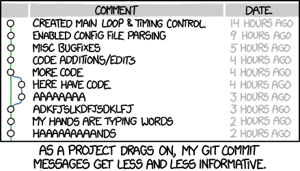
Do not let this happen to your code!

Tip

Read this guide on how to write better commit messages.

Git Workflows

A Git Workflow is a recipe or recommendation for how to use git to accomplish work in a consistent and productive manner. Given git’s focus on flexibility, there is no standardized process on how to interact with git. These workflows ensure that all the developers in a team are making changes to the project in a uniform fashion. It is important to note that these workflows are more guidelines than strict rules.

Popular git workflows

1. Centralized workflow
2. Feature branch workflow
3. Gitflow
4. Forking workflow

You can read more about these over here. In the hands-on workshop task you will be using the feature branch workflow.

Version control for large files

git is decentralized, which means that changes in large files cause git repositories to grow by the size of the file (not by the size of the change) every time the file is committed. Luckily, there are multiple third party implementations that will try to solve the problem, many of them use similar paradigms to provide solutions.

There are many routes one could go through to achieve this result. Some of them are mentioned below:

1. git-lfs: Git Large File Storage works by storing a pointer to the file in the git repository instead of the file itself. The blobs are written to a separate server using the Git LFS HTTP API. Hence, in order to use git-lfs your repository hosting platform must support it. Fortunately, GitHub, BitBucket and GitLab all support git-lfs. Learn more here.
2. git-annex: Git-annex works by storing the contents of files being tracked by it to separate location. What is stored into the repository, is a symlink to the to the key under the separate location. In order to share the large binary files between a team for example the tracked files need to be stored to a different backend (like Amazon S3). Note that GitHub does not support git-annex (i.e. you cannot use GitHub as a backend) but GitLab does. Learn more here.
3. dat Dat is a nonprofit-backed community & open protocol for building apps of the future. Use Dat command line to share files with version control, back up data to servers, browse remote files on demand, and automate long-term data preservation. Dat allows you to Track your files with automatic version history, share files with others over a secure peer to peer network and automate live backups to external HDs or remote servers. Learn more here.

The easiest way to get started with versioning your large file is by using git-lfs, but git-annex and dat offer more flexibility and are more modern options.

Source Code Hosting

What is GitHub?

GitHub is a web-based hosting service for version control using Git. It offers all of the distributed version control and source code management (SCM) functionality of Git as well as adding its own features. It provides access control and several collaboration features such as bug tracking, feature requests, task management, and wikis for every project GitHub offers plans for both private repositories and free accounts which are commonly used to host open-source software projects.

Exercise

1. Create a GitHub account
2. Get familiar with GitHub
3. Read this short guide

SSH vs HTTPS

The connection to the server is secured with SSH or HTTPS. GitHub explains which URL to use. If you use SSH you will need an SSH key. Read here to learn how to connect to GitHub with SSH.

When using your_username to clone/fetch a repository from the_author, an SSH url will look like:

git@github.com:[the_author]/[repository].git

and HTTPS will look like:

https://[your_username]@github.com/[the_author]/[repository].git.

Semantic versioning

Have you ever wondered how developers decide how to number the different versions of their software? Do they just randomly come up with numbers? No, the version number consists of 3 numbers, x.y.z where x is a major change, y is a minor change and z a patch. There is official documentation on this, which you can read if you are interested. But assume you have a tool that reads some data and performs some function on the data. If you find a bug and fix it, you publish the fix by adding to z. If you added a small functionality, for example support for compressed data input and compatibility with other tools, increase y. If you added another function to it, increase x.

Licensing

Public repositories on GitHub are often used to share open source software. For your repository to truly be open source, you’ll need to license it so that others are free to use, change, and distribute the software. You’re under no obligation to choose a license. However, without a license, the default copyright laws apply, meaning that you retain all rights to your source code and no one may reproduce, distribute, or create derivative works from your work.

For example: if you use GitHub and/or Bitbucket, you can publish your tool with the GNU licensing. GNU is open source, and open source does not mean free. Whenever using code with GNU licensing, you must cite the authors/developers. For more information on the license check the GNU organization documentation.

This link contains useful information to help you choose a license for your project.

README and Markdown syntax

It’s a good practice to make a README for your repository. The README file can also be edited online using the editors GitHub and Bitbucket provide. Typically they are written in Markdown syntax, which is very simple. You might have heard about R Markdown, but Markdown is a syntax that R has knitted into its compiler. Again there are many tutorials to learn Markdown. You can check the syntax on the Atlassian website.

A README should include information about:

• name of the tool and the version
• what is this tool about
• who are the authors
• requirements and dependencies
• how to install/clone it
• how to run it
• what is the input and output
• licensing
• how to cite it

Look at this nice outline for a standard README file in Markdown syntax. To get the source code click the Raw button on the top left.

Bug and Issue tracking

Both GitHub and Bitbucket allow for issue tracking. Members of a team can create an issue, assign it to a developer or admin, and comment on it. An issue can be marked according to its importance and type, for example, fixing a bug or adding functionality; and the issue can be resolved once it is has been taken care of. Issues can be linked to commits, to show which commit resulted in resolving an issue.

When a repository is publicly accessible, you can create issues to inform the developers there is a bug or a functionality you would be interested in. So, the next time you find an issue with some tool that you can’t resolve after trying for a few days, just post an issue on their GitHub repository. You can also link/mention issues and commits from different repositories.

Read this useful guide to learn more.

Workshop 7. Version Control with git workshop

Instructors: Dileep Kishore and Dakota Hawkins

In this workshop you will work on both basic and advanced git commands and collaborate with each other through git repositories. For this workshop you will be working in small teams of 2-3 people. You can either complete the tasks on the Shared Computing Cluster (SCC) or on your local computer. We will be using the git command line interface throughout this workshop.

Tip

To login to the SCC use: ssh <username>@scc1.bu.edu

Getting started

You will be working on a movie recommender system that recommends movies based on plot and keyword similarities.

Task 1

1. One team member should fork this repository: https://github.com/dileep-kishore/git-intro
2. Add all your other team members as collaborators.
3. Clone the repository
4. Follow the instructions in the README to set up your environment
5. Ensure that the package runs as expected

Tip

1. If you’re working on the scc you can use module load anaconda3
2. Look at the git history
3. Observe the list of remote repositories

Your first contribution

You can now make your first contribution to the package

Task 2

1. Add your name to the contributors section of the README
2. Commit your changes
3. Oops, I meant to ask you to add your team member’s name not yours. Fix that.
4. Push, pull and merge (fix conflicts, if any)

Tip

1. If you’re stuck, look up how to ammend a commit
2. Use git status to explore what happens to the unstaged and staging areas

Exploring the tree

In this section you will explore the history of the repository

Task 3

1. Go back 10-20 commits (these should be one of my commits)
2. Now go to commit 0338440
3. What’s changed?
4. Compare the version of the README you had just updated with this version
5. Go back to the latest commit

Extending the source code

Software development usually involves multiple developers working on the software at the same time. You will now divide your team into bug fixers and feature contributors. Don’t worry you will get to switch roles in the middle.

Task 4

1. Bug fixers (will work on the master branch)

   • Fix: Raise ValueError when unsupported method is passed to movie_recommender
   • Now switch roles
   • Fix: Load pickled recommender when available

2. Feature contributors (will create a new feature branch)

   • Feat: Save the recommender object after training
   • Now switch roles
   • Feat: Unknown movie query returns fuzzy matches

The save, load and search functions are already implemented in utils.py and can be imported as

``from .utils import save, load, search``

Tip

1. How can the bug fixers also get access to the feature branch?
2. Make sure you merge to master after completing your first feature
3. Use git stash to stash changes before switching branches

Changing history

When you git a time-machine the first thing you do is go change history.

Task 5

1. Reset the repository to the state it was in when you found it (my last commit). Observe the working directory
2. Now reset it back to your commit
3. Now revert your last commit. Observe the git history
4. Undo your revert

Caution

Do not push or pull if you’ve just reset to a previous commit. This will screw up your history and make things a lot more complicated since the remote history will be different.

Tip

1. Use git reflog to get the reference of your last commit before you reset
2. Can you reset a revert?

Getting ready for the release

Task 6

1. Add the pickled file to gitignore. We don’t want to store binaries in version control especially large binaries.
2. Tag your commit with a version number. Finally, release your source code.

Send me a pull request

You can inform other’s of you magnificent changes and accomplishments by making pull requests. This way you let everyone know that you made some changes and they need to pull.

Task 7

Create a new pull request.

Tip

Ideally pull requests should be from branches in your fork of the repository

Schedule

The workshops for summer 2018 meet on the following dates:

• Friday, August 10 9-11AM (CILSE 106B): Intro to linux and command line
• Monday, August 13 9-11AM (CILSE 106B): Intro to python
• Wednesday, August 15 9-11AM (CILSE 106B): Real world application workshop 1
• Friday, August 17 9-11AM (LSEB 904): Intro to R <– Note different location!
• Monday, August 20 9-11AM (CILSE 106B): Advanced linux command line tools
• Wednesday, August 22 9-11AM (CILSE 106B): Real world application workshop 2
• Wednesday, October 24th 12-2PM (LSE 904): Shell scripting and cluster computing
• Wednesday, November 7th 12-2PM (LSE 904): Version control with git

Contents

• Workshop 0 - CLI Basics
• Workshop 1 - python
• Workshop 2 - High throughput sequencing application
• Workshop 3 - Advanced CLI
• Workshop 4 - Introduction to R
• Workshop 5 - High throughput sequencing application part 2
• Workshop 6 - Shell scripting and cluster computing
• Workshop 7 - Version Control with git

List of topics

Note

These workshops are still under construction Please be kind.

Workshop 0 - CLI Basics

Workshop 0. Basic Linux and Command Line Usage: Online Materials

Workshop 0. Basic Linux and Command Line Usage: Workshop

Topic	Length
CLI Introduction	3 min
Navigating directories, listing files	16 min
Basic file operations	9 min
Working with files 1	10 min
Working with files 2	10 min
I/O redirection and related commands	20 min
Globbing	6 min

Workshop 1 - python

Workshop 1. Introduction to Python

Workshop 1: Protein Translation using Python

Topic	Length
Introduction	3 min
Builtin Types	2 min
A Simple Program	6 min
if Statements	3 min
Simplifying Solution	4 min
Defining Functions	4 min
More On Types and Iteration	4 min
More Data Structures
File I/O	22 min
Modules	3 min
Executing Scripts with Arguments from the Command Line	3 min
Other File objects

Workshop 2 - High throughput sequencing application

Workshop 2. High Throughput Sequencing Application Session Online Materials

Workshop 2. High Throughput Sequencing Application Session

Topic	Length
App Session Introduction	2 min
Illumina Sequencing Technology	5 min
High Throughput Sequencing Data Primer	9 min
Sequencing Data QC and Analysis Primer	9 min

Workshop 3 - Advanced CLI

Workshop 3. Advanced CLI and Tools

Workshop 3. Advanced CLI Techniques Workshop Session

Topic	Length
nano	~7 min
vim (part one, two, three)	~9, ~6, ~6 min
emacs	~24 min
piping, silencing stdout/stderr	~10 min
shell tricks	~10 min
bash history	~4 min
pushd/popd, find, xargs/fim	~10 min

Workshop 4 - Introduction to R

Workshop 4. Introduction to R

Workshop 4. Introduction to R

Topic	Length
Reasons why you should learn R	~7 min
RStudio interface	~10 min
Installing packages	~7 min
Console and working environment basics	~8 min
Very quick data types	~7 min
NAs, NaNs, Infs	~3 min
Intro to vectors	~7 min
Data types and structures, Part 2	9:30 min
If statements and logical operators	5:30 min
Apply function	~7 min
Reshape package	~6 min
Split, Apply and Combine with plyr	8:30 min
Intro to ggplot	9 min

Workshop 5 - High throughput sequencing application part 2

Workshop 5. NGS Application Session 2

Workshop 5. NGS Application Session 2 Workshop

There are no video online materials for this workshop.

Workshop 6 - Shell scripting and cluster computing

Workshop 6. Shell Scripts and Cluster Computing

There is no in-class workshop material for this workshop.

Workshop 7 - Version control with git

Workshop 7. Version Control with git

Workshop 7. Version Control with git workshop

---

Contributors

The primary contributors to the BU Bioinformatics Programming Workshop Taskforce:

• Gracia Bonilla
• Rachael Ivison
• Vinay Kartha
• Josh Klein
• Adam Labadorf
• Katharine Norwood

We would also like to thank Gary Benson for his mentorship and support.

Indices and tables

• Index
• Module Index
• Search Page